
-
admin wrote a new post 1 week, 6 days ago
Nano Banana 2 vs Nano Banana Pro: What’s the Difference?Nano Banana Pro has been my personal favorite tool for creating high-quality social media […]
-
admin wrote a new post 1 week, 6 days ago
Our agreement with the Department of WarDetails on OpenAI’s contract with the Department of War, outlining safety red lines, legal protections, and how AI systems will be deployed in classified environments.
-
admin wrote a new post 1 week, 6 days ago
-
admin wrote a new post 1 week, 6 days ago
-
admin wrote a new post 2 weeks ago
Joint Statement from OpenAI and MicrosoftMicrosoft and OpenAI continue to work closely across research, engineering, and product development, building on years of deep collaboration and shared success.
-
admin wrote a new post 2 weeks ago
Mercury 2: The AI Model That Feels InstantYou must have faced the never-ending wait of an AI model taking its time to answer your query. To put an […]
-
admin wrote a new post 2 weeks ago
Google Launches Nano Banana 2: Learn All About It!Nano Banana! The image model that took the world by storm just got eclipsed by…itself. Yes! G […]
-
admin wrote a new post 2 weeks ago
How to Build Interactive Geospatial Dashboards Using Folium with Heatmaps, Choropleths, Time Animation, Marker Clustering, and Advanced Interactive Plugins
 In this Folium tutorial, we build a complete set of interactive maps that run in Colab or any local Python setup. We explore multiple basemap styles, design rich markers with HTML popups, and visualize spatial density using heatmaps. We also create region-level choropleth maps from GeoJSON, scale to thousands of points using marker clustering, and animate time-based movement with a timestamped layer. Finally, we combine real-world USGS earthquake data with layered magnitude buckets, density heatmaps, legends, and fullscreen controls to produce a practical, dashboard-like global monitor. Copy CodeCopiedUse a different Browserimport folium from folium import plugins from folium.plugins import HeatMap, MarkerCluster, TimestampedGeoJson, MiniMap, Draw, Fullscreen import pandas as pd import numpy as np import json import requests from datetime import datetime, timedelta import branca.colormap as cm print(f”Folium version: {folium.__version__}”) print(“All imports successful!n”) We import all required libraries, such as Folium, Pandas, NumPy, Requests, and Folium plugins to prepare our geospatial environment. We initialize the mapping workflow by confirming the Folium version and ensuring that all dependencies load successfully. This setup establishes the technical foundation for building interactive maps, processing data, and integrating external geospatial sources. Copy CodeCopiedUse a different Browserdef create_multi_tile_map(): “””Create a map with multiple tile layers””” m = folium.Map( location=[40.7128, -74.0060], zoom_start=12, tiles=’OpenStreetMap’ ) folium.TileLayer(‘cartodbpositron’, name=’CartoDB Positron’).add_to(m) folium.TileLayer(‘cartodbdark_matter’, name=’CartoDB Dark Matter’).add_to(m) folium.TileLayer( tiles=’https://tiles.stadiamaps.com/tiles/stamen_terrain/{z}/{x}/{y}.png’, attr=’Map tiles by Stamen Design, under CC BY 3.0. Data by OpenStreetMap, under ODbL’, name=’Terrain’ ).add_to(m) folium.TileLayer( tiles=’https://tiles.stadiamaps.com/tiles/stamen_toner/{z}/{x}/{y}.png’, attr=’Map tiles by Stamen Design, under CC BY 3.0. Data by OpenStreetMap, under ODbL’, name=’Toner’ ).add_to(m) folium.TileLayer( tiles=’https://tiles.stadiamaps.com/tiles/stamen_watercolor/{z}/{x}/{y}.jpg’, attr=’Map tiles by Stamen Design, under CC BY 3.0. Data by OpenStreetMap, under ODbL’, name=’Watercolor’ ).add_to(m) folium.LayerControl().add_to(m) return m We create a multi-layer base map and configure multiple tile providers to enable different visual styles. We add terrain, dark mode, toner, and watercolor layers so we can switch perspectives based on the analytical requirements. By including a layer control panel, we can dynamically toggle map styles and explore spatial data more effectively. Copy CodeCopiedUse a different Browserdef create_advanced_markers_map(): “””Create map with custom markers and HTML popups””” landmarks = [ {‘name’: ‘Statue of Liberty’, ‘lat’: 40.6892, ‘lon’: -74.0445, ‘type’: ‘monument’, ‘visitors’: 4500000}, {‘name’: ‘Empire State Building’, ‘lat’: 40.7484, ‘lon’: -73.9857, ‘type’: ‘building’, ‘visitors’: 4000000}, {‘name’: ‘Central Park’, ‘lat’: 40.7829, ‘lon’: -73.9654, ‘type’: ‘park’, ‘visitors’: 42000000}, {‘name’: ‘Brooklyn Bridge’, ‘lat’: 40.7061, ‘lon’: -73.9969, ‘type’: ‘bridge’, ‘visitors’: 4000000}, {‘name’: ‘Times Square’, ‘lat’: 40.7580, ‘lon’: -73.9855, ‘type’: ‘plaza’, ‘visitors’: 50000000} ] m = folium.Map(location=[40.7128, -74.0060], zoom_start=12) icon_colors = { ‘monument’: ‘red’, ‘building’: ‘blue’, ‘park’: ‘green’, ‘bridge’: ‘orange’, ‘plaza’: ‘purple’ } icon_symbols = { ‘monument’: ‘star’, ‘building’: ‘home’, ‘park’: ‘tree’, ‘bridge’: ‘road’, ‘plaza’: ‘shopping-cart’ } for landmark in landmarks: html = f””” {landmark[‘name’]} Type: {landmark[‘type’].title()} Annual Visitors: {landmark[‘visitors’]:,} “”” iframe = folium.IFrame(html, width=220, height=250) popup = folium.Popup(iframe, max_width=220) folium.Marker( location=[landmark[‘lat’], landmark[‘lon’]], popup=popup, tooltip=landmark[‘name’], icon=folium.Icon( color=icon_colors[landmark[‘type’]], icon=icon_symbols[landmark[‘type’]], prefix=’fa’ ) ).add_to(m) folium.CircleMarker( location=[40.7128, -74.0060], radius=20, popup=’NYC Center’, color=’#3186cc’, fill=True, fillColor=’#3186cc’, fillOpacity=0.2 ).add_to(m) return m We build a map with advanced markers and rich HTML popups to represent real-world landmarks. We customize marker icons, colors, and symbols by location type to enhance visual clarity and semantic meaning. By embedding structured HTML content inside popups, we present detailed contextual information directly within the interactive map. Copy CodeCopiedUse a different Browserdef create_heatmap(): “””Create a heatmap showing data density””” np.random.seed(42) n_incidents = 1000 crime_data = [] hotspots = [ [40.7580, -73.9855], [40.7484, -73.9857], [40.7128, -74.0060], ] for _ in range(n_incidents): hotspot = hotspots[np.random.choice(len(hotspots))] lat = hotspot[0] + np.random.normal(0, 0.02) lon = hotspot[1] + np.random.normal(0, 0.02) intensity = np.random.uniform(0.3, 1.0) crime_data.append([lat, lon, intensity]) m = folium.Map(location=[40.7128, -74.0060], zoom_start=12) HeatMap( crime_data, min_opacity=0.2, max_zoom=18, max_val=1.0, radius=15, blur=25, gradient={ 0.0: ‘blue’, 0.3: ‘lime’, 0.5: ‘yellow’, 0.7: ‘orange’, 1.0: ‘red’ } ).add_to(m) title_html = ”’ NYC Crime Density Heatmap Simulated incident data ”’ m.get_root().html.add_child(folium.Element(title_html)) return m We generate synthetic spatial data and use a heatmap to visualize density patterns across geographic locations. We simulate clustered coordinates and apply gradient-based intensity visualization to reveal spatial concentration trends. By overlaying this density layer on the map, we gain insight into how events distribute across regions. Copy CodeCopiedUse a different Browserdef create_choropleth_map(): “””Create a choropleth map showing data across regions””” us_states_url = ‘https://raw.githubusercontent.com/python-visualization/folium/master/examples/data/us-states.json’ try: us_states = requests.get(us_states_url).json() except: print(“Warning: Could not fetch GeoJSON data. Using offline sample.”) return None state_data = { ‘Alabama’: 5.1, ‘Alaska’: 6.3, ‘Arizona’: 4.7, ‘Arkansas’: 3.8, ‘California’: 5.3, ‘Colorado’: 3.9, ‘Connecticut’: 4.3, ‘Delaware’: 4.1, ‘Florida’: 3.6, ‘Georgia’: 4.0, ‘Hawaii’: 2.8, ‘Idaho’: 2.9, ‘Illinois’: 5.0, ‘Indiana’: 3.5, ‘Iowa’: 3.1, ‘Kansas’: 3.3, ‘Kentucky’: 4.3, ‘Louisiana’: 4.6, ‘Maine’: 3.2, ‘Maryland’: 4.0, ‘Massachusetts’: 3.6, ‘Michigan’: 4.3, ‘Minnesota’: 3.2, ‘Mississippi’: 5.2, ‘Missouri’: 3.7, ‘Montana’: 3.5, ‘Nebraska’: 2.9, ‘Nevada’: 4.8, ‘New Hampshire’: 2.7, ‘New Jersey’: 4.2, ‘New Mexico’: 5.0, ‘New York’: 4.5, ‘North Carolina’: 4.0, ‘North Dakota’: 2.6, ‘Ohio’: 4.2, ‘Oklahoma’: 3.4, ‘Oregon’: 4.2, ‘Pennsylvania’: 4.4, ‘Rhode Island’: 4.0, ‘South Carolina’: 3.5, ‘South Dakota’: 2.9, ‘Tennessee’: 3.6, ‘Texas’: 4.0, ‘Utah’: 2.8, ‘Vermont’: 2.8, ‘Virginia’: 3.3, ‘Washington’: 4.6, ‘West Virginia’: 5.1, ‘Wisconsin’: 3.4, ‘Wyoming’: 3.6 } df = pd.DataFrame(list(state_data.items()), columns=[‘State’, ‘Unemployment’]) m = folium.Map(location=[37.8, -96], zoom_start=4) folium.Choropleth( geo_data=us_states, name=’choropleth’, data=df, columns=[‘State’, ‘Unemployment’], key_on=’feature.properties.name’, fill_color=’YlOrRd’, fill_opacity=0.7, line_opacity=0.5, legend_name=’Unemployment Rate (%)’ ).add_to(m) style_function = lambda x: {‘fillColor’: ‘#ffffff’, ‘color’:’#000000′, ‘fillOpacity’: 0.1, ‘weight’: 0.1} highlight_function = lambda x: {‘fillColor’: ‘#000000’, ‘color’:’#000000′, ‘fillOpacity’: 0.50, ‘weight’: 0.1} NIL = folium.features.GeoJson( us_states, style_function=style_function, control=False, highlight_function=highlight_function, tooltip=folium.features.GeoJsonTooltip( fields=[‘name’], aliases=[‘State:’], style=(“background-color: white; color: #333333; font-family: arial; font-size: 12px; padding: 10px;”) ) ) m.add_child(NIL) m.keep_in_front(NIL) folium.LayerControl().add_to(m) return m We create a choropleth map by combining GeoJSON boundary data with structured numerical attributes. We map unemployment rates to geographic regions and use color gradients to visually represent statistical differences. By enabling hover interactions and tooltips, we can explore region-specific data directly within the map interface. Copy CodeCopiedUse a different Browserdef create_marker_cluster_map(): “””Create a map with marker clustering for large datasets””” np.random.seed(123) n_locations = 5000 lats = np.random.uniform(25, 49, n_locations) lons = np.random.uniform(-125, -65, n_locations) values = np.random.randint(1, 100, n_locations) df_markers = pd.DataFrame({ ‘lat’: lats, ‘lon’: lons, ‘value’: values }) m = folium.Map(location=[37.8, -96], zoom_start=4) marker_cluster = MarkerCluster( name=’Location Cluster’, overlay=True, control=True ).add_to(m) for idx, row in df_markers.iterrows(): if row[‘value’] < 33: color = 'green' elif row['value'] < 66: color = 'orange' else: color = 'red' folium.Marker( location=[row['lat'], row['lon']], popup=f"Value: {row['value']}", tooltip=f"Location {idx}", icon=folium.Icon(color=color, icon='info-sign') ).add_to(marker_cluster) folium.LayerControl().add_to(m) title_html = ''' Marker Clustering Demo 5000 markers – zoom to see individual points ''' m.get_root().html.add_child(folium.Element(title_html)) return m def create_time_series_map(): """Create an animated map showing data changes over time""" start_date = datetime(2024, 8, 1) features = [] path = [ [25.0, -70.0], [26.5, -72.0], [28.0, -74.5], [29.5, -76.5], [31.0, -78.0], [32.5, -79.5], [34.0, -80.5], [35.5, -81.0] ] for i, (lat, lon) in enumerate(path): timestamp = start_date + timedelta(hours=i*6) feature = { 'type': 'Feature', 'geometry': { 'type': 'Point', 'coordinates': [lon, lat] }, 'properties': { 'time': timestamp.isoformat(), 'popup': f'Hurricane PositionTime: {timestamp.strftime("%Y-%m-%d %H:%M")}Category: {min(5, i//2 + 1)}', 'icon': 'circle', 'iconstyle': { 'fillColor': ['yellow', 'orange', 'red', 'darkred', 'purple'][min(4, i//2)], 'fillOpacity': 0.8, 'stroke': 'true', 'radius': 8 + i * 2 } } } features.append(feature) m = folium.Map( location=[30.0, -75.0], zoom_start=5, tiles='CartoDB Positron' ) TimestampedGeoJson( {'type': 'FeatureCollection', 'features': features}, period='PT6H', add_last_point=True, auto_play=True, loop=True, max_speed=2, loop_button=True, date_options='YYYY-MM-DD HH:mm', time_slider_drag_update=True ).add_to(m) title_html = ''' Hurricane Path Animation Simulated hurricane tracking Use controls below to play/pause ''' m.get_root().html.add_child(folium.Element(title_html)) return m def create_interactive_plugins_map(): """Create a map with multiple interactive plugins""" m = folium.Map( location=[40.7128, -74.0060], zoom_start=12, tiles='OpenStreetMap' ) minimap = MiniMap(toggle_display=True) m.add_child(minimap) draw = Draw( export=True, filename='drawn_shapes.geojson', position='topleft', draw_options={ 'polyline': True, 'polygon': True, 'circle': True, 'rectangle': True, 'marker': True, 'circlemarker': True }, edit_options={'edit': True} ) m.add_child(draw) Fullscreen( position='topright', title='Expand map', title_cancel='Exit fullscreen', force_separate_button=True ).add_to(m) plugins.MeasureControl( position='bottomleft', primary_length_unit='kilometers', secondary_length_unit='miles', primary_area_unit='sqkilometers', secondary_area_unit='acres' ).add_to(m) plugins.MousePosition( position='bottomright', separator=' | ', empty_string='NaN', lng_first=True, num_digits=20, prefix='Coordinates:', ).add_to(m) plugins.LocateControl( auto_start=False, position='topleft' ).add_to(m) folium.Marker( [40.7128, -74.0060], popup='NYCTry the drawing tools!', icon=folium.Icon(color='red', icon='info-sign') ).add_to(m) return m def create_earthquake_map(): """Create comprehensive earthquake visualization using real USGS data""" url = 'https://earthquake.usgs.gov/earthquakes/feed/v1.0/summary/2.5_month.geojson' try: response = requests.get(url) earthquake_data = response.json() print(f"Successfully loaded {len(earthquake_data['features'])} earthquakes") except Exception as e: print(f"Error fetching data: {e}") earthquake_data = { 'features': [ { 'properties': {'mag': 5.2, 'place': 'Sample Location 1', 'time': 1640000000000}, 'geometry': {'coordinates': [-122.0, 37.0, 10]} }, { 'properties': {'mag': 6.1, 'place': 'Sample Location 2', 'time': 1640100000000}, 'geometry': {'coordinates': [140.0, 35.0, 20]} } ] } earthquakes = [] for feature in earthquake_data['features']: props = feature['properties'] coords = feature['geometry']['coordinates'] earthquakes.append({ 'lat': coords[1], 'lon': coords[0], 'depth': coords[2], 'magnitude': props.get('mag', 0), 'place': props.get('place', 'Unknown'), 'time': datetime.fromtimestamp(props.get('time', 0) / 1000) }) df_eq = pd.DataFrame(earthquakes) print(f"nEarthquake Statistics:") print(f"Total earthquakes: {len(df_eq)}") print(f"Magnitude range: {df_eq['magnitude'].min():.1f} – {df_eq['magnitude'].max():.1f}") print(f"Depth range: {df_eq['depth'].min():.1f} – {df_eq['depth'].max():.1f} km") m = folium.Map( location=[20, 0], zoom_start=2, tiles='CartoDB dark_matter' ) minor = folium.FeatureGroup(name='Minor (< 4.0)') moderate = folium.FeatureGroup(name='Moderate (4.0-5.0)') strong = folium.FeatureGroup(name='Strong (5.0-6.0)') major = folium.FeatureGroup(name='Major (≥ 6.0)') for idx, eq in df_eq.iterrows(): mag = eq['magnitude'] if mag < 4.0: color = 'green' radius = 3 group = minor elif mag < 5.0: color = 'yellow' radius = 6 group = moderate elif mag < 6.0: color = 'orange' radius = 9 group = strong else: color = 'red' radius = 12 group = major popup_html = f""" Magnitude {mag:.1f} Location: {eq['place']} Depth: {eq['depth']:.1f} km Time: {eq['time'].strftime('%Y-%m-%d %H:%M:%S')} Coordinates: {eq['lat']:.4f}, {eq['lon']:.4f} """ folium.CircleMarker( location=[eq['lat'], eq['lon']], radius=radius, popup=folium.Popup(popup_html, max_width=270), tooltip=f"M{mag:.1f} – {eq['place']}", color=color, fill=True, fillColor=color, fillOpacity=0.7, weight=2 ).add_to(group) minor.add_to(m) moderate.add_to(m) strong.add_to(m) major.add_to(m) heat_data = [[row['lat'], row['lon'], row['magnitude']] for idx, row in df_eq.iterrows()] heatmap = folium.FeatureGroup(name='Density Heatmap', show=False) HeatMap( heat_data, min_opacity=0.3, radius=15, blur=20, gradient={0.4: 'blue', 0.6: 'cyan', 0.7: 'lime', 0.8: 'yellow', 1: 'red'} ).add_to(heatmap) heatmap.add_to(m) folium.LayerControl(position='topright', collapsed=False).add_to(m) legend_html = ''' Earthquake Magnitude ● Minor (< 4.0) ● Moderate (4.0-5.0) ● Strong (5.0-6.0) ● Major (≥ 6.0) Data: USGS (Past 30 days) ''' m.get_root().html.add_child(folium.Element(legend_html)) title_html = ''' Global Earthquake Monitor Real-time earthquake data (M ≥ 2.5) Click markers for details | Toggle layers to explore ''' m.get_root().html.add_child(folium.Element(title_html)) Fullscreen(position='topright').add_to(m) return m if __name__ == "__main__": print("=" * 80) print("ADVANCED FOLIUM TUTORIAL – ALL EXAMPLES") print("=" * 80) print("nGenerating all maps…n") maps = { 'multi_tile_map': create_multi_tile_map(), 'advanced_markers_map': create_advanced_markers_map(), 'heatmap': create_heatmap(), 'choropleth_map': create_choropleth_map(), 'marker_cluster_map': create_marker_cluster_map(), 'time_series_map': create_time_series_map(), 'interactive_plugins_map': create_interactive_plugins_map(), 'earthquake_map': create_earthquake_map() } print("n" + "=" * 80) print("SAVING MAPS TO HTML FILES") print("=" * 80) for name, map_obj in maps.items(): if map_obj is not None: filename = f"{name}.html" map_obj.save(filename) print(f"✓ Saved: {filename}") else: print(f"✗ Skipped: {name} (map generation failed)") print("n" + "=" * 80) print("ALL MAPS GENERATED SUCCESSFULLY!") print("=" * 80) print("nYou can now:") print("1. Open any HTML file in your browser to view the interactive map") print("2. Access the map objects in code using the 'maps' dictionary") print("3. Display maps in Jupyter/Colab by returning the map object") print("nExample: To display the earthquake map in a notebook, just run:") print(" maps['earthquake_map']") print("n" + "=" * 80) We implement advanced geospatial features, including marker clustering, time-series animation, interactive plugins, and real-world earthquake visualization. We integrate live USGS data, categorize earthquakes by magnitude, and enhance interpretation using feature groups, heatmaps, and custom legends. By combining interactivity, animation, and real-data integration, we build a comprehensive, production-ready geospatial visualization system. In conclusion, we have a reusable Folium “toolbox” that covers both core mapping patterns and production-style interactivity. We generated and saved multiple maps as standalone HTML files, making them easy to share, embed, or iterate on without extra infrastructure. We also demonstrated how to move from synthetic demo data to live public feeds while keeping the visualization structured with layers, tooltips, pop-ups, and controls. Also, we can confidently extend the script by plugging in our own datasets, adding new GeoJSON boundaries, enriching popups with charts or images, and turning Folium maps into lightweight geospatial applications. Check out the Full Codes here . Also, feel free to follow us on Twitter and don’t forget to join our 120k+ ML SubReddit and Subscribe to our Newsletter. Wait! are you on telegram? now you can join us on telegram as well. The post How to Build Interactive Geospatial Dashboards Using Folium with Heatmaps, Choropleths, Time Animation, Marker Clustering, and Advanced Interactive Plugins appeared first on MarkTec […]
 -
admin wrote a new post 2 weeks ago
Sakana AI Introduces Doc-to-LoRA and Text-to-LoRA: Hypernetworks that Instantly Internalize Long Contexts and Adapt LLMs via Zero-Shot Natural Language
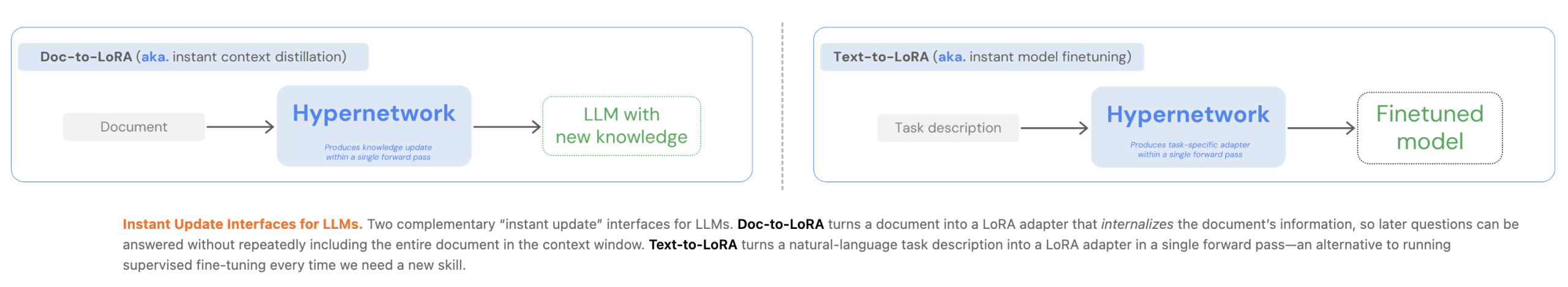 Customizing Large Language Models (LLMs) currently presents a significant engineering trade-off between the flexibility of In-Context Learning (ICL) and the efficiency of Context Distillation (CD) or Supervised Fine-Tuning (SFT). Tokyo-based Sakana AI has proposed a new approach to bypass these constraints through cost amortization. In two of their recent papers, they introduced Text-to-LoRA (T2L) and Doc-to-LoRA (D2L), lightweight hypernetworks that meta-learn to generate Low-Rank Adaptation (LoRA) matrices in a single forward pass. The Engineering Bottleneck: Latency vs. Memory For AI Devs, the primary limitation of standard LLM adaptation is computational overhead: In-Context Learning (ICL): While convenient, ICL suffers from quadratic attention costs and linear KV-cache growth, which increases latency and memory consumption as prompts lengthen. Context Distillation (CD): CD transfers information into model parameters, but per-prompt distillation is often impractical due to high training costs and update latency. SFT: Requires task-specific datasets and expensive re-training if information changes. Sakana AI’s methods amortize these costs by paying a one-time meta-training fee. Once trained, the hypernetwork can instantly adapt the base LLM to new tasks or documents without additional backpropagation. Text-to-LoRA (T2L): Adaptation via Natural Language Text-to-LoRA (T2L) is a hypernetwork designed to adapt LLMs on the fly using only a natural language description of a task. Architecture and Training T2L uses a task encoder to extract vector representations from text descriptions. This representation, combined with learnable module and layer embeddings, is processed through a series of MLP blocks to generate the A and B low-rank matrices for the target LLM. The system can be trained via two primary schemes: LoRA Reconstruction: Distilling existing, pre-trained LoRA adapters into the hypernetwork. Supervised Fine-Tuning (SFT): Optimizing the hypernetwork end-to-end on multi-task datasets. The research indicates that SFT-trained T2L generalizes better to unseen tasks because it implicitly learns to cluster related functionalities in weight space. In benchmarks, T2L matched or outperformed task-specific adapters on tasks like GSM8K and Arc-Challenge, while reducing adaptation costs by over 4x compared to 3-shot ICL. Doc-to-LoRA (D2L): Internalizing Context Doc-to-LoRA (D2L) extends this concept to document internalization. It enables an LLM to answer subsequent queries about a document without re-consuming the original context, effectively removing the document from the active context window. Perceiver-Based Design D2L utilizes a Perceiver-style cross-attention architecture. It maps variable-length token activations (Z) from the base LLM into a fixed-shape LoRA adapter. To handle documents exceeding the training length, D2L employs a chunking mechanism. Long contexts are partitioned into K contiguous chunks, each processed independently to produce per-chunk adapters. These are then concatenated along the rank dimension, allowing D2L to generate higher-rank LoRAs for longer inputs without changing the hypernetwork’s output shape. Performance and Memory Efficiency On a Needle-in-a-Haystack (NIAH) retrieval task, D2L maintained near-perfect zero-shot accuracy on context lengths exceeding the base model’s native window by more than 4x. Memory Impact: For a 128K-token document, a base model requires over 12 GB of VRAM for the KV cache. Internalized D2L models handled the same document using less than 50 MB. Update Latency: D2L internalizes information in sub-s […]
 -
admin wrote a new post 2 weeks ago
How to Run a Collaborative Giveaway on Instagram Running a giveaway on social media is not a new concept. But running a collaborative giveaway, together with a brand or your bestie? Now, that’s a…
-
admin wrote a new post 2 weeks ago
76% of Shoppers Fear AI Misinformation on Business Websites: Here’s How to Build a Chatbot They’ll Trust
 Your shoppers are nervous. And they have good […]
 -
admin wrote a new post 2 weeks ago
MIT Technology Review is a 2026 ASME finalist in reportingThe American Society of Magazine Editors has named MIT Technology Review as a finalist […]
-
admin wrote a new post 2 weeks ago
The Download: how AI is shaking up Go, and a cybersecurity mystery
 This is today’s edition of The Download, our weekday newsletter that provides a d […]
 -
admin wrote a new post 2 weeks ago
Scaling AI for everyoneToday we’re announcing $110B in new investment at a $730B pre money valuation. This includes $30B from SoftBank, $30B from NVIDIA, and $50B from Amazon.
-
admin wrote a new post 2 weeks ago
Introducing the Stateful Runtime Environment for Agents in Amazon BedrockStateful Runtime for Agents in Amazon Bedrock brings persistent orchestration, memory, and secure execution to multi-step AI workflows powered by OpenAI.
-
admin wrote a new post 2 weeks ago
OpenAI and Amazon announce strategic partnershipOpenAI and Amazon announce a strategic partnership bringing OpenAI’s Frontier platform to AWS, expanding AI infrastructure, custom models, and enterprise AI agents.
-
admin wrote a new post 2 weeks ago
-
admin wrote a new post 2 weeks ago
AI is rewiring how the world’s best Go players thinkBurrowed in the alleys of Hongik-dong, a hushed residential neighborhood in eastern Seoul, is […]
-
admin wrote a new post 2 weeks ago
Nano Banana 2: Google’s latest AI image generation modelNano Banana! The image model that took the world by storm just got eclipsed by…itself. Y […]
-
admin wrote a new post 2 weeks ago
Excel 101: Complete Guide to VLOOKUP FunctionTry the following – ask any Excel user for his/ her favourite Excel formula. More often than not, y […]
- Load More
admin
Last active: Active 3 months ago
SHARE:
Comments: 0
Likes: 0
Submitted: 1044
Friends: 0
User Rating: Be the first one!
Adsterra
🔥 Top Offers (Limited Time)