A Coding Implementation of a Complete Hierarchical Bayesian Regression Workflow in NumPyro Using JAX-Powered Inference and Posterior Predictive AnalysisIn this tutorial, we explore hierarchical Bayesian regression with NumPyro and walk through the entire workflow in a structured manner. We start by generating synthetic data, then we define a probabilistic model that captures both global patterns and group-level variations. Through each snippet, we set up inference using NUTS, analyze posterior distributions, and perform posterior predictive checks to understand how well our model captures the underlying structure. By approaching the tutorial step by step, we build an intuitive understanding of how NumPyro enables flexible, scalable Bayesian modeling. Check out the Full Codes here. Copy CodeCopiedUse a different Browsertry: import numpyro except ImportError: !pip install -q “llvmlite>=0.45.1” “numpyro[cpu]” matplotlib pandas import numpy as np import pandas as pd import matplotlib.pyplot as plt import jax import jax.numpy as jnp from jax import random import numpyro import numpyro.distributions as dist from numpyro.infer import MCMC, NUTS, Predictive from numpyro.diagnostics import hpdi numpyro.set_host_device_count(1) We set up our environment by installing NumPyro and importing all required libraries. We prepare JAX, NumPyro, and plotting tools so we have everything ready for Bayesian inference. As we run this cell, we ensure our Colab session is fully equipped for hierarchical modeling. Check out the Full Codes here. Copy CodeCopiedUse a different Browserdef generate_data(key, n_groups=8, n_per_group=40): k1, k2, k3, k4 = random.split(key, 4) true_alpha = 1.0 true_beta = 0.6 sigma_alpha_g = 0.8 sigma_beta_g = 0.5 sigma_eps = 0.7 group_ids = np.repeat(np.arange(n_groups), n_per_group) n = n_groups * n_per_group alpha_g = random.normal(k1, (n_groups,)) * sigma_alpha_g beta_g = random.normal(k2, (n_groups,)) * sigma_beta_g x = random.normal(k3, (n,)) * 2.0 eps = random.normal(k4, (n,)) * sigma_eps a = true_alpha + alpha_g[group_ids] b = true_beta + beta_g[group_ids] y = a + b * x + eps df = pd.DataFrame({“y”: np.array(y), “x”: np.array(x), “group”: group_ids}) truth = dict(true_alpha=true_alpha, true_beta=true_beta, sigma_alpha_group=sigma_alpha_g, sigma_beta_group=sigma_beta_g, sigma_eps=sigma_eps) return df, truth key = random.PRNGKey(0) df, truth = generate_data(key) x = jnp.array(df[“x”].values) y = jnp.array(df[“y”].values) groups = jnp.array(df[“group”].values) n_groups = int(df[“group”].nunique()) We generate synthetic hierarchical data that mimics real-world group-level variation. We convert this data into JAX-friendly arrays so NumPyro can process it efficiently. By doing this, we lay the foundation for fitting a model that learns both global trends and group differences. Check out the Full Codes here. Copy CodeCopiedUse a different Browserdef hierarchical_regression_model(x, group_idx, n_groups, y=None): mu_alpha = numpyro.sample(“mu_alpha”, dist.Normal(0.0, 5.0)) mu_beta = numpyro.sample(“mu_beta”, dist.Normal(0.0, 5.0)) sigma_alpha = numpyro.sample(“sigma_alpha”, dist.HalfCauchy(2.0)) sigma_beta = numpyro.sample(“sigma_beta”, dist.HalfCauchy(2.0)) with numpyro.plate(“group”, n_groups): alpha_g = numpyro.sample(“alpha_g”, dist.Normal(mu_alpha, sigma_alpha)) beta_g = numpyro.sample(“beta_g”, dist.Normal(mu_beta, sigma_beta)) sigma_obs = numpyro.sample(“sigma_obs”, dist.Exponential(1.0)) alpha = alpha_g[group_idx] beta = beta_g[group_idx] mean = alpha + beta * x with numpyro.plate(“data”, x.shape[0]): numpyro.sample(“y”, dist.Normal(mean, sigma_obs), obs=y) nuts = NUTS(hierarchical_regression_model, target_accept_prob=0.9) mcmc = MCMC(nuts, num_warmup=1000, num_samples=1000, num_chains=1, progress_bar=True) mcmc.run(random.PRNGKey(1), x=x, group_idx=groups, n_groups=n_groups, y=y) samples = mcmc.get_samples() We define our hierarchical regression model and launch the NUTS-based MCMC sampler. We allow NumPyro to explore the posterior space and learn parameters such as group intercepts and slopes. As this sampling completes, we obtain rich posterior distributions that reflect uncertainty at every level. Check out the Full Codes here. Copy CodeCopiedUse a different Browserdef param_summary(arr): arr = np.asarray(arr) mean = arr.mean() lo, hi = hpdi(arr, prob=0.9) return mean, float(lo), float(hi) for name in [“mu_alpha”, “mu_beta”, “sigma_alpha”, “sigma_beta”, “sigma_obs”]: m, lo, hi = param_summary(samples[name]) print(f”{name}: mean={m:.3f}, HPDI=[{lo:.3f}, {hi:.3f}]”) predictive = Predictive(hierarchical_regression_model, samples, return_sites=[“y”]) ppc = predictive(random.PRNGKey(2), x=x, group_idx=groups, n_groups=n_groups) y_rep = np.asarray(ppc[“y”]) group_to_plot = 0 mask = df[“group”].values == group_to_plot x_g = df.loc[mask, “x”].values y_g = df.loc[mask, “y”].values y_rep_g = y_rep[:, mask] order = np.argsort(x_g) x_sorted = x_g[order] y_rep_sorted = y_rep_g[:, order] y_med = np.median(y_rep_sorted, axis=0) y_lo, y_hi = np.percentile(y_rep_sorted, [5, 95], axis=0) plt.figure(figsize=(8, 5)) plt.scatter(x_g, y_g) plt.plot(x_sorted, y_med) plt.fill_between(x_sorted, y_lo, y_hi, alpha=0.3) plt.show() We analyze our posterior samples by computing summaries and performing posterior predictive checks. We visualize how well the model recreates observed data for a selected group. This step helps us understand how accurately our model captures the underlying generative process. Check out the Full Codes here. Copy CodeCopiedUse a different Browseralpha_g = np.asarray(samples[“alpha_g”]).mean(axis=0) beta_g = np.asarray(samples[“beta_g”]).mean(axis=0) fig, axes = plt.subplots(1, 2, figsize=(12, 4)) axes[0].bar(range(n_groups), alpha_g) axes[0].axhline(truth[“true_alpha”], linestyle=”–“) axes[1].bar(range(n_groups), beta_g) axes[1].axhline(truth[“true_beta”], linestyle=”–“) plt.tight_layout() plt.show() We plot the estimated group-level intercepts and slopes to compare their learned patterns with the true values. We explore how each group behaves and how the model adapts to their differences. This final visualization brings together the complete picture of hierarchical inference. In conclusion, we implemented how NumPyro allows us to model hierarchical relationships with clarity, efficiency, and strong expressive power. We observed how the posterior results reveal meaningful global and group-specific effects, and how predictive checks validate the model’s fit to the generated data. As we put everything together, we gain confidence in constructing, fitting, and interpreting hierarchical models using JAX-powered inference. This process strengthens our ability to apply Bayesian thinking to richer, more realistic datasets where multilevel structure is essential. Check out the Full Codes here. Feel free to check out our GitHub Page for Tutorials, Codes and Notebooks. Also, feel free to follow us on Twitter and don’t forget to join our 100k+ ML SubReddit and Subscribe to our Newsletter. Wait! are you on telegram? now you can join us on telegram as well. The post A Coding Implementation of a Complete Hierarchical Bayesian Regression Workflow in NumPyro Using JAX-Powered Inference and Posterior Predictive Analysis appeared first on M […]

Microsoft AI Releases VibeVoice-Realtime: A Lightweight Real‑Time Text-to-Speech Model Supporting Streaming Text Input and Robust Long-Form Speech GenerationMicrosoft has released VibeVoice-Realtime-0.5B, a real time text to speech model that works with streaming text input and long form speech output, aimed at agent style applications and live data narration. The model can start producing audible speech in about 300 ms, which is critical when a language model is still generating the rest of its answer. Where VibeVoice Realtime Fits in the VibeVoice Stack? VibeVoice is a broader framework that focuses on next token diffusion over continuous speech tokens, with variants designed for long form multi speaker audio such as podcasts. The research team shows that the main VibeVoice models can synthesize up to 90 minutes of speech with up to 4 speakers in a 64k context window using continuous speech tokenizers at 7.5 Hz. The Realtime 0.5B variant is the low latency branch of this family. The model card reports an 8k context length and a typical generation length of about 10 minutes for a single speaker, which is enough for most voice agents, system narrators and live dashboards. A separate set of VibeVoice models, VibeVoice-1.5B and VibeVoice Large, handle long form multi speaker audio with 32k and 64k context windows and longer generation times. Interleaved Streaming Architecture The realtime variant uses an interleaved windowed design. Incoming text is split into chunks. The model incrementally encodes new text chunks while, in parallel, continuing diffusion based acoustic latent generation from prior context. This overlap between text encoding and acoustic decoding is what lets the system reach about 300 ms first audio latency on suitable hardware. Unlike the long form VibeVoice variants, which use both semantic and acoustic tokenizers, the realtime model removes the semantic tokenizer and uses only an acoustic tokenizer that operates at 7.5 Hz. The acoustic tokenizer is based on a σ VAE variant from LatentLM, with a mirror symmetric encoder decoder architecture that uses 7 stages of modified transformer blocks and performs 3200x downsampling from 24 kHz audio. On top of this tokenizer, a diffusion head predicts acoustic VAE features. The diffusion head has 4 layers and about 40M parameters and is conditioned on hidden states from Qwen2.5-0.5B. It uses a Denoising Diffusion Probabilistic Models process with Classifier Free Guidance and DPM Solver style samplers, following the next token diffusion approach of the full VibeVoice system. Training proceeds in two stages. First, the acoustic tokenizer is pre trained. Then the tokenizer is frozen and the team trains the LLM along with the diffusion head with curriculum learning on sequence length, increasing from about 4k to 8,192 tokens. This keeps the tokenizer stable, while the LLM and diffusion head learn to map from text tokens to acoustic tokens across long contexts. Quality on LibriSpeech and SEED The VibeVoice Realtime reports zero shot performance on LibriSpeech test clean. VibeVoice Realtime 0.5B reaches word error rate (WER) 2.00 percent and speaker similarity 0.695. For comparison, VALL-E 2 has WER 2.40 with similarity 0.643 and Voicebox has WER 1.90 with similarity 0.662 on the same benchmark. On the SEED test benchmark for short utterances, VibeVoice Realtime-0.5B reaches WER 2.05 percent and speaker similarity 0.633. SparkTTS gets a slightly lower WER 1.98 but lower similarity 0.584, while Seed TTS reaches WER 2.25 and the highest reported similarity 0.762. The research team noted that the realtime model is optimized for long form robustness, so short sentence metrics are informative but not the main target. From an engineering point of view, the interesting part is the tradeoff. By running the acoustic tokenizer at 7.5 Hz and using next token diffusion, the model reduces the number of steps per second of audio compared to higher frame rate tokenizers, while preserving competitive WER and speaker similarity. Integration Pattern for Agents And Applications The recommended setup is to run VibeVoice-Realtime-0.5B next to a conversational LLM. The LLM streams tokens during generation. These text chunks feed directly into the VibeVoice server, which synthesizes audio in parallel and streams it back to the client. For many systems this looks like a small microservice. The TTS process has a fixed 8k context and about 10 minutes of audio budget per request, which fits typical agent dialogs, support calls and monitoring dashboards. Because the model is speech only and does not generate background ambience or music, it is better suited for voice interfaces, assistant style products and programmatic narration rather than media production. Key Takeaways Low latency streaming TTS: VibeVoice-Realtime-0.5B is a real time text to speech model that supports streaming text input and can emit the first audio frames in about 300 ms, which makes it suitable for interactive agents and live narration where users cannot tolerate 1 to 3 second delays. LLM along with diffusion over continuous speech tokens: The model follows the VibeVoice design, it uses a Qwen2.5 0.5B language model to process text context and dialogue flow, then a diffusion head operates on continuous acoustic tokens from a low frame rate tokenizer to generate waveform level detail, which scales better to long sequences than classic spectrogram based TTS. Around 1B total parameters with acoustic stack: While the base LLM has 0.5B parameters, the acoustic decoder has about 340M parameters and the diffusion head about 40M parameters, so the full realtime stack is roughly 1B parameters, which is important for GPU memory planning and deployment sizing. Competitive quality on LibriSpeech and SEED: On LibriSpeech test clean, VibeVoice-Realtime-0.5B reaches word error rate 2.00 percent and speaker similarity 0.695, and on SEED test en it reaches 2.05 percent WER and 0.633 similarity, which places it in the same quality band as strong recent TTS systems while still being tuned for long form robustness. Check out the Model Card on HF. Feel free to check out our GitHub Page for Tutorials, Codes and Notebooks. Also, feel free to follow us on Twitter and don’t forget to join our 100k+ ML SubReddit and Subscribe to our Newsletter. Wait! are you on telegram? now you can join us on telegram as well. The post Microsoft AI Releases VibeVoice-Realtime: A Lightweight Real‑Time Text-to-Speech Model Supporting Streaming Text Input and Robust Long-Form Speech Generation appeared […]

How to Build an Adaptive Meta-Reasoning Agent That Dynamically Chooses Between Fast, Deep, and Tool-Based Thinking Strategies We begin this tutorial […]

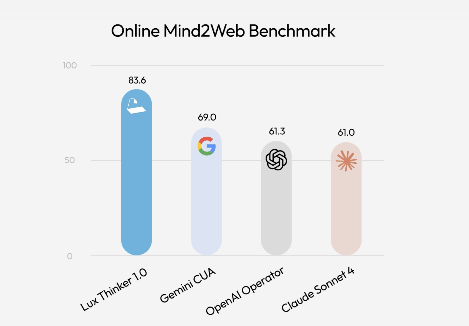
OpenAGI Foundation Launches Lux: A Foundation Computer Use Model that Tops Online Mind2Web with OSGym At Scale How do you turn slow, manual click […]

Kernel Principal Component Analysis (PCA): Explained with an Example 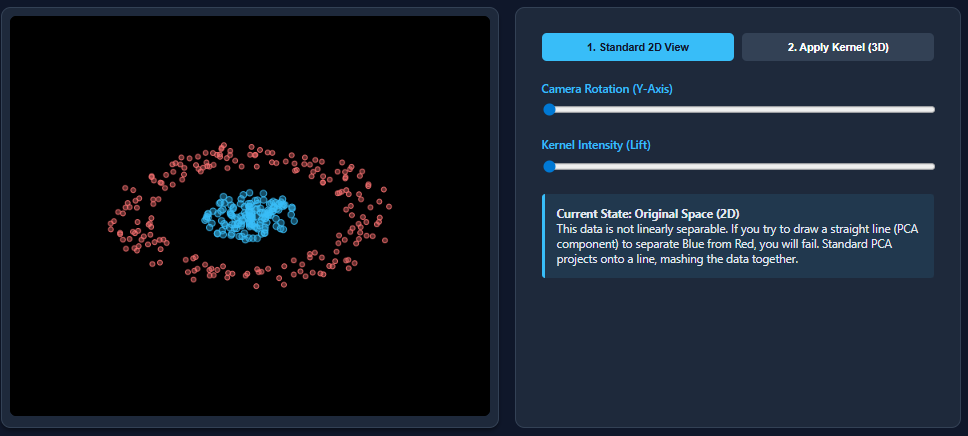Dimensionality reduction techniques like PCA work wonderfully when datasets are […]

How to Design a Fully Local Multi-Agent Orchestration System Using TinyLlama for Intelligent Task Decomposition and Autonomous Collaboration In […]

Apple Researchers Release CLaRa: A Continuous Latent Reasoning Framework for Compression‑Native RAG with 16x–128x Semantic Document Compression 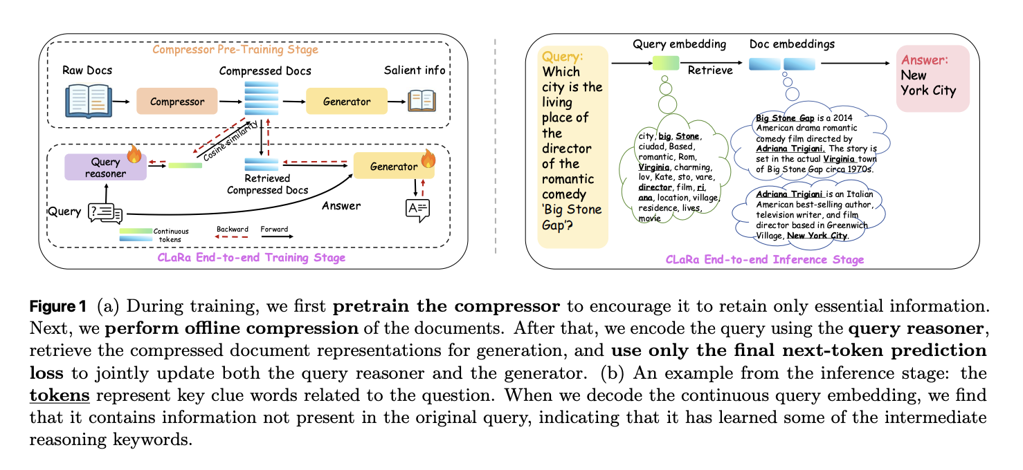How do you keep RAG systems accurate and efficient when every query tries to stuff thousands of tokens into the context window and the retriever and generator are still optimized as 2 separate, disconnected systems? A team of researchers from Apple and University of Edinburgh released CLaRa, Continuous Latent Reasoning, (CLaRa-7B-Base, CLaRa-7B-Instruct and CLaRa-7B-E2E) a retrieval augmented generation framework that compresses documents into continuous memory tokens and then performs both retrieval and generation in that shared latent space. The goal is simple. Shorten context, avoid double encoding, and let the generator teach the retriever what actually matters for downstream answers. From raw documents to continuous memory tokens CLaRa starts with a semantic compressor that attaches a small number of learned memory tokens to each document. During Salient Compressor Pretraining, SCP, the base model is a Mistral 7B style transformer with LoRA adapters that switch between a compressor role and a generator role. The final layer hidden states of the memory tokens become the compressed representation for that document. SCP is trained on about 2M passages from Wikipedia 2021. A local Qwen-32B model generates 3 supervision signals for each passage. Simple QA pairs cover atomic facts. Complex QA pairs connect several facts in one question to enforce multi hop reasoning. Paraphrases reorder and compress the text while preserving semantics. A verification loop checks factual consistency and coverage and can regenerate missing questions or paraphrases for up to 10 rounds before accepting a sample. Training uses 2 losses. A cross entropy term trains the generator to answer questions or produce paraphrases conditioned only on the memory tokens and an instruction prefix. A mean squared error term aligns the average hidden state of document tokens with the average hidden state of the memory tokens. The MSE loss gives modest but consistent gains of about 0.3 to 0.6 F1 points at compression ratios 32 and 128 and keeps compressed and original representations in the same semantic region. Joint retrieval and generation in a shared space After offline compression, each document is represented only by its memory tokens. CLaRa then trains a query reasoner and an answer generator on top of the same backbone. The query reasoner is another LoRA adapter that maps an input question into the same number of memory tokens used for documents. Retrieval becomes pure embedding search. The system computes cosine similarity between the query embedding and each candidate document embedding. The best compressed document embeddings for a query are concatenated with the query tokens and fed into the generator adapter. Training uses only a standard next token prediction loss on the final answer. There are no explicit relevance labels. The key trick is a differentiable top k selector implemented with a Straight Through estimator. During the forward pass the model uses hard top k selection. During the backward pass a softmax distribution over document scores allows gradients from the generator to flow into the query reasoner parameters. The research team shows 2 effects in the gradient analysis. First, the retriever is encouraged to assign higher probability to documents that increase answer likelihood. Second, because retrieval and generation share the same compressed representations, generator gradients reshape the latent document space to make it easier to reason over. Logit lens analysis of the query embeddings recovers topic tokens such as “NFL” and “Oklahoma” for a question about the nephew of Ivory Lee Brown, even though those tokens are not in the raw query but are present in the supporting articles. Compression quality and QA accuracy The compressor is evaluated on 4 QA datasets: Natural Questions, HotpotQA, MuSiQue and 2WikiMultihopQA. Under the Normal setting, where the system retrieves the top 5 Wikipedia 2021 documents per query, SCP-Mistral-7B at 4 times compression reaches an average F1 of 39.86. This is 5.37 points better than the hard compression baseline LLMLingua 2 and 1.13 points better than the best soft compression baseline PISCO. Under the Oracle setting, where the gold document is guaranteed to be in the candidate set, SCP-Mistral-7B at 4 times compression reaches an average F1 of 66.76. That is 17.31 points above LLMLingua-2 and 5.35 points above PISCO. Even more interesting, the compressed representations outperform a BGE based text retriever plus full document Mistral-7B generator by about 2.36 average F1 points for Mistral and about 6.36 points for Phi 4 mini. Well trained soft compression can exceed full text RAG while cutting context length by factors from 4 to 128. The performance at very high compression ratios, above 32 in Oracle, does drop, but the decline remains moderate in Normal retrieval conditions. The key explanation as per the research team is, weak document relevance bottlenecks the system before compression quality does. End to end QA and retrieval behavior For end to end QA, CLaRa uses 20 candidate documents per query with compression ratios 4, 16 and 32. On the Normal setting, CLaRa-Mistral-7B with instruction initialized weights and 16 times compression reaches F1 equal to 50.89 on Natural Questions and 44.66 on 2WikiMultihopQA. This is comparable to DRO-Mistral-7B, which reads full uncompressed text, while using 16 times shorter document representations. On some datasets, CLaRa at 16 times compression slightly improves F1 over DRO, for example from 43.65 to 47.18 on 2Wiki. In the Oracle setting, CLaRa-Mistral-7B exceeds 75, F1 on both Natural Questions and HotpotQA at 4 times compression. This shows that the generator can fully exploit accurate retrieval even when all evidence is stored only in compressed memory tokens. Instruction initialized CLaRa generally wins over pre-training initialized CLaRa in the Normal setting, while the gap narrows in Oracle, where retrieval noise is limited. On the retrieval side, CLaRa used as a reranker under Oracle conditions delivers strong Recall at 5. With pretraining initialization at compression 4 on HotpotQA, CLaRa-Mistral-7B reaches Recall at 5 equal to 96.21. This beats the supervised BGE Reranker baseline at 85.93 by 10.28 points and even outperforms a fully supervised Sup Instruct retriever trained with contrastive relevance labels. What Apple has released? Apple’s research team released 3 models on Hugging Face: CLaRa-7B-Base, CLaRa-7B-Instruct and CLaRa-7B-E2E. CLaRa-7B-Instruct is described as an instruction tuned unified RAG model with built in document compression at 16 and 128 times. It answers instruction style questions directly from compressed representations and uses Mistral-7B-Instruct v0.2 as the base model. Key Takeaways CLaRa replaces raw documents with a small set of continuous memory tokens learned via QA guided and paraphrase guided semantic compression, which preserves key reasoning signals even at 16 times and 128 times compression. Retrieval and generation are trained in a single shared latent space, the query encoder and generator share the same compressed representations and are optimized together with one language modeling loss. A differentiable top-k estimator lets gradients flow from answer tokens back into the retriever, which aligns document relevance with answer quality and removes the usual disjoint tuning loop for RAG systems. On multi hop QA benchmarks like Natural Questions, HotpotQA, MuSiQue and 2WikiMultihopQA, CLaRa’s SCP compressor at 4 times compression outperforms strong text based baselines such as LLMLingua 2 and PISCO and can even beat full text BGE/ Mistral pipelines on average F1. Apple has released 3 practical models, CLaRa-7B-Base, CLaRa-7B-Instruct and CLaRa-7B-E2E, along with the full training pipeline on GitHub. Editorial Notes CLaRa is an important step for retrieval augmented generation because it treats semantic document compression and joint optimization in a shared continuous space as first class citizens, not afterthoughts bolted onto a text only pipeline. It shows that embedding based compression with SCP, combined with end to end training via a differentiable top-k estimator and a single language modeling loss, can match or surpass text based RAG baselines while using far shorter contexts and simpler retrieval stacks. Overall, CLaRa demonstrates that unified continuous latent reasoning is a credible alternative to classic chunk and retrieve RAG for real world QA workloads. Check out the Paper, Model Weights on HF and Repo. Feel free to check out our GitHub Page for Tutorials, Codes and Notebooks. Also, feel free to follow us on Twitter and don’t forget to join our 100k+ ML SubReddit and Subscribe to our Newsletter. Wait! are you on telegram? now you can join us on telegram as well. The post Apple Researchers Release CLaRa: A Continuous Latent Reasoning Framework for Compression‑Native RAG with 16x–128x Semantic Document Compression appeared first o […]

K-Means Cluster Evaluation with Silhouette AnalysisClustering models in machine learning must be assessed by how well they separate data into meaningful groups with distinctive characteristics.

The Complete Guide to Docker for Machine Learning EngineersMachine learning models often behave differently across environments.

Preparing Data for BERT TrainingThis article is divided into four parts; they are: • Preparing Documents • Creating Sentence Pairs from Doc […]

BERT Models and Its VariantsThis article is divided into two parts; they are: • Architecture and Training of BERT • Variations of BERT BERT is an encoder-only model.

From Shannon to Modern AI: A Complete Information Theory Guide for Machine Learning  In 1948, Claude Shannon published a paper that changed how we think about information forever.

Why Decision Trees Fail (and How to Fix Them)  Decision tree-based models for predictive machine learning tasks like classification and regression […]

Training a Tokenizer for BERT ModelsThis article is divided into two parts; they are: • Picking a Dataset • Training a Tokenizer To keep things simple, we’ll use English text only.

Forecasting the Future with Tree-Based Models for Time SeriesDecision tree-based models in machine learning are frequently used for a wide range of predictive tasks such as classification and regression, typically on structured, tabular data.

The Complete AI Agent Decision FrameworkYou’ve learned about

Mastering JSON Prompting for LLMsLLMs

ACMA SMS Sender ID Register: What You Need to Know Please note: The regulatory environment for SMS Sender ID registration in Australia is evolving, […]

Black Friday Marketing: SMS or Email? Black Friday… It’s the time of year many retail organisations pin their hopes on. When inboxes overflow wit […]

How to Get the Blue Tick on WhatsApp in 2025 Meta recently changed its WhatsApp verified badge from a green tick to a blue tick, aligning it with […]