Z.ai debuts open source GLM-4.6V, a native tool-calling vision model for multimodal reasoningChinese AI startup Zhipu AI aka Z.ai has released its […]

Subliminal Learning: How AI Models Inherit Hidden DangersResearchers have uncovered an unexpected flaw in one of the most common techniques used […]

Agent Frameworks vs Runtime vs Harnesses: What They Are and When to Use Which AI agents are LLM-powered systems that act autonomously to solve […]

Jina AI Releases Jina-VLM: A 2.4B Multilingual Vision Language Model Focused on Token Efficient Visual QA 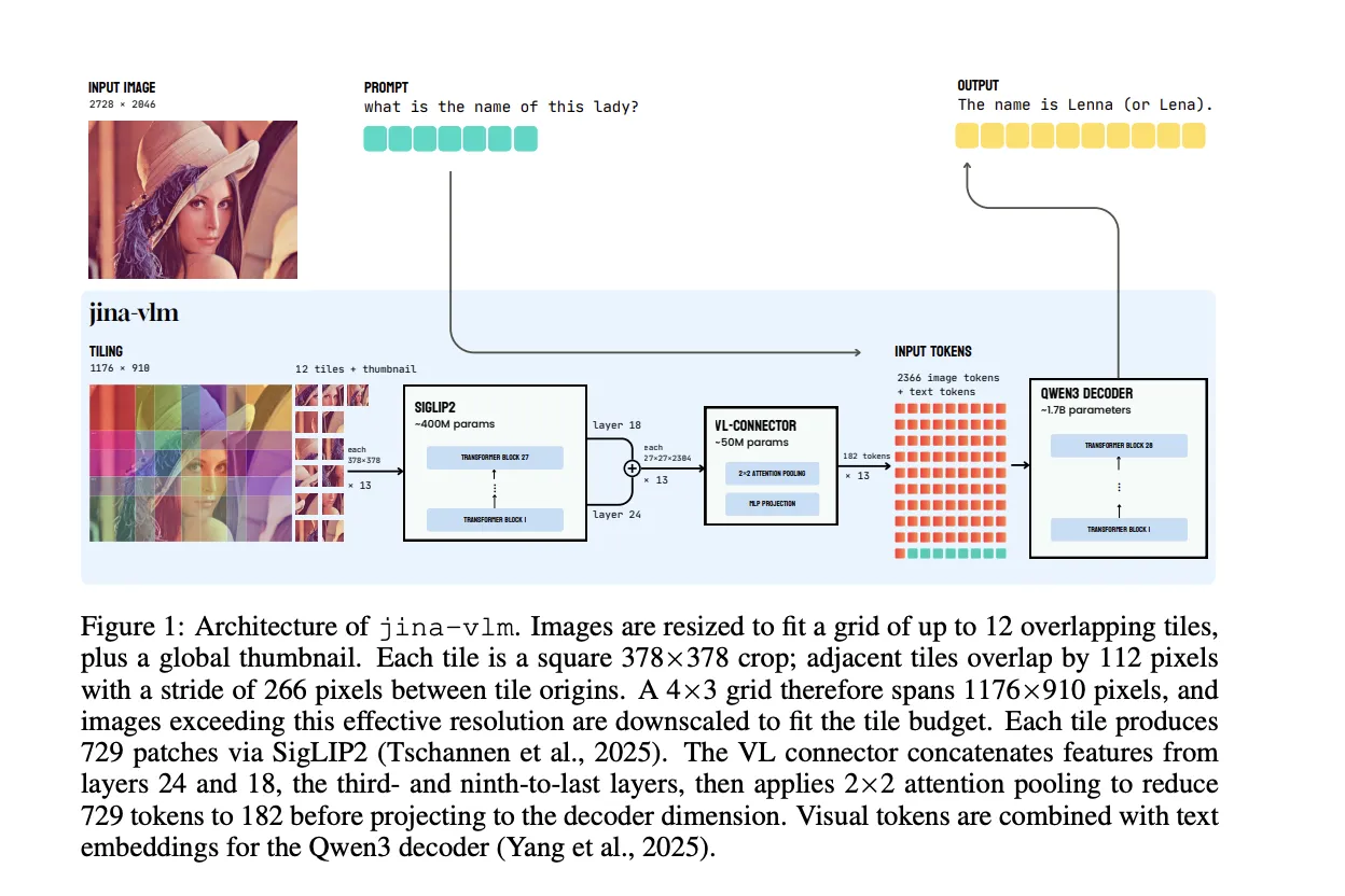Jina AI has released Jina-VLM, a 2.4B […]

Interview: From CUDA to Tile-Based Programming: NVIDIA’s Stephen Jones on Building the Future of AI As AI models grow in complexity and hardware […]

Carousel, Reel, or Feed Post? When to Use Each Instagram Content FormatYou’re working on your content calendar. You’ve got the ideas, but now you need to choose a format. “Should it be a video? A gallery? Maybe…

The State of AI: A vision of the world in 2030Welcome back to The State of AI, a new collaboration between the Financial Times and MIT Technology […]

The Download: four (still) big breakthroughs, and how our bodies fare in extreme heat This is today’s edition of The Download, our weekday new […]

Anthropic's Claude Code can now read your Slack messages and write code for youAnthropic on Monday launched a beta integration that connects its […]

Booking.com’s agent strategy: Disciplined, modular and already delivering 2× accuracyWhen many enterprises weren’t even thinking about agentic b […]

Instacart and OpenAI partner on AI shopping experiencesOpenAI and Instacart are deepening their longstanding partnership by bringing the first fully integrated grocery shopping and Instant Checkout payment app to ChatGPT.

Design in the age of AI: How small businesses are building big brands fasterPresented by Design.comFor most of history, design was the last step […]

The state of enterprise AIKey findings from OpenAI’s enterprise data show accelerating AI adoption, deeper integration, and measurable productivity gains across industries in 2025.

4 technologies that didn’t make our 2026 breakthroughs listIf you’re a longtime reader, you probably know that our newsroom selects 10 b […]

From Transformers to Associative Memory, How Titans and MIRAS Rethink Long Context Modeling 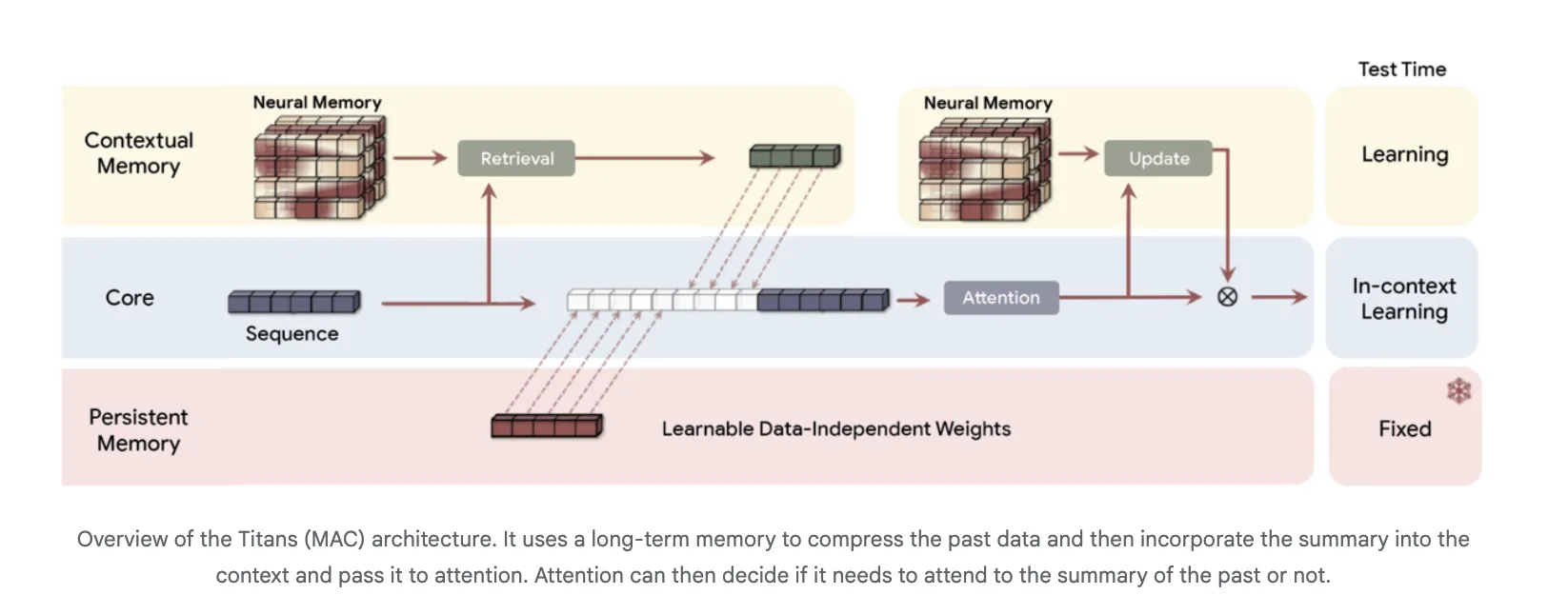What comes after Transformers? Google Research is […]

Cisco Released Cisco Time Series Model: Their First Open-Weights Foundation Model based on Decoder-only Transformer Architecture Cisco and Splunk […]

Google Colab Integrates KaggleHub for One Click Access to Kaggle Datasets, Models and CompetitionsGoogle is closing an old gap between Kaggle and […]

A Coding Implementation of a Complete Hierarchical Bayesian Regression Workflow in NumPyro Using JAX-Powered Inference and Posterior Predictive AnalysisIn this tutorial, we explore hierarchical Bayesian regression with NumPyro and walk through the entire workflow in a structured manner. We start by generating synthetic data, then we define a probabilistic model that captures both global patterns and group-level variations. Through each snippet, we set up inference using NUTS, analyze posterior distributions, and perform posterior predictive checks to understand how well our model captures the underlying structure. By approaching the tutorial step by step, we build an intuitive understanding of how NumPyro enables flexible, scalable Bayesian modeling. Check out the Full Codes here. Copy CodeCopiedUse a different Browsertry: import numpyro except ImportError: !pip install -q “llvmlite>=0.45.1” “numpyro[cpu]” matplotlib pandas import numpy as np import pandas as pd import matplotlib.pyplot as plt import jax import jax.numpy as jnp from jax import random import numpyro import numpyro.distributions as dist from numpyro.infer import MCMC, NUTS, Predictive from numpyro.diagnostics import hpdi numpyro.set_host_device_count(1) We set up our environment by installing NumPyro and importing all required libraries. We prepare JAX, NumPyro, and plotting tools so we have everything ready for Bayesian inference. As we run this cell, we ensure our Colab session is fully equipped for hierarchical modeling. Check out the Full Codes here. Copy CodeCopiedUse a different Browserdef generate_data(key, n_groups=8, n_per_group=40): k1, k2, k3, k4 = random.split(key, 4) true_alpha = 1.0 true_beta = 0.6 sigma_alpha_g = 0.8 sigma_beta_g = 0.5 sigma_eps = 0.7 group_ids = np.repeat(np.arange(n_groups), n_per_group) n = n_groups * n_per_group alpha_g = random.normal(k1, (n_groups,)) * sigma_alpha_g beta_g = random.normal(k2, (n_groups,)) * sigma_beta_g x = random.normal(k3, (n,)) * 2.0 eps = random.normal(k4, (n,)) * sigma_eps a = true_alpha + alpha_g[group_ids] b = true_beta + beta_g[group_ids] y = a + b * x + eps df = pd.DataFrame({“y”: np.array(y), “x”: np.array(x), “group”: group_ids}) truth = dict(true_alpha=true_alpha, true_beta=true_beta, sigma_alpha_group=sigma_alpha_g, sigma_beta_group=sigma_beta_g, sigma_eps=sigma_eps) return df, truth key = random.PRNGKey(0) df, truth = generate_data(key) x = jnp.array(df[“x”].values) y = jnp.array(df[“y”].values) groups = jnp.array(df[“group”].values) n_groups = int(df[“group”].nunique()) We generate synthetic hierarchical data that mimics real-world group-level variation. We convert this data into JAX-friendly arrays so NumPyro can process it efficiently. By doing this, we lay the foundation for fitting a model that learns both global trends and group differences. Check out the Full Codes here. Copy CodeCopiedUse a different Browserdef hierarchical_regression_model(x, group_idx, n_groups, y=None): mu_alpha = numpyro.sample(“mu_alpha”, dist.Normal(0.0, 5.0)) mu_beta = numpyro.sample(“mu_beta”, dist.Normal(0.0, 5.0)) sigma_alpha = numpyro.sample(“sigma_alpha”, dist.HalfCauchy(2.0)) sigma_beta = numpyro.sample(“sigma_beta”, dist.HalfCauchy(2.0)) with numpyro.plate(“group”, n_groups): alpha_g = numpyro.sample(“alpha_g”, dist.Normal(mu_alpha, sigma_alpha)) beta_g = numpyro.sample(“beta_g”, dist.Normal(mu_beta, sigma_beta)) sigma_obs = numpyro.sample(“sigma_obs”, dist.Exponential(1.0)) alpha = alpha_g[group_idx] beta = beta_g[group_idx] mean = alpha + beta * x with numpyro.plate(“data”, x.shape[0]): numpyro.sample(“y”, dist.Normal(mean, sigma_obs), obs=y) nuts = NUTS(hierarchical_regression_model, target_accept_prob=0.9) mcmc = MCMC(nuts, num_warmup=1000, num_samples=1000, num_chains=1, progress_bar=True) mcmc.run(random.PRNGKey(1), x=x, group_idx=groups, n_groups=n_groups, y=y) samples = mcmc.get_samples() We define our hierarchical regression model and launch the NUTS-based MCMC sampler. We allow NumPyro to explore the posterior space and learn parameters such as group intercepts and slopes. As this sampling completes, we obtain rich posterior distributions that reflect uncertainty at every level. Check out the Full Codes here. Copy CodeCopiedUse a different Browserdef param_summary(arr): arr = np.asarray(arr) mean = arr.mean() lo, hi = hpdi(arr, prob=0.9) return mean, float(lo), float(hi) for name in [“mu_alpha”, “mu_beta”, “sigma_alpha”, “sigma_beta”, “sigma_obs”]: m, lo, hi = param_summary(samples[name]) print(f”{name}: mean={m:.3f}, HPDI=[{lo:.3f}, {hi:.3f}]”) predictive = Predictive(hierarchical_regression_model, samples, return_sites=[“y”]) ppc = predictive(random.PRNGKey(2), x=x, group_idx=groups, n_groups=n_groups) y_rep = np.asarray(ppc[“y”]) group_to_plot = 0 mask = df[“group”].values == group_to_plot x_g = df.loc[mask, “x”].values y_g = df.loc[mask, “y”].values y_rep_g = y_rep[:, mask] order = np.argsort(x_g) x_sorted = x_g[order] y_rep_sorted = y_rep_g[:, order] y_med = np.median(y_rep_sorted, axis=0) y_lo, y_hi = np.percentile(y_rep_sorted, [5, 95], axis=0) plt.figure(figsize=(8, 5)) plt.scatter(x_g, y_g) plt.plot(x_sorted, y_med) plt.fill_between(x_sorted, y_lo, y_hi, alpha=0.3) plt.show() We analyze our posterior samples by computing summaries and performing posterior predictive checks. We visualize how well the model recreates observed data for a selected group. This step helps us understand how accurately our model captures the underlying generative process. Check out the Full Codes here. Copy CodeCopiedUse a different Browseralpha_g = np.asarray(samples[“alpha_g”]).mean(axis=0) beta_g = np.asarray(samples[“beta_g”]).mean(axis=0) fig, axes = plt.subplots(1, 2, figsize=(12, 4)) axes[0].bar(range(n_groups), alpha_g) axes[0].axhline(truth[“true_alpha”], linestyle=”–“) axes[1].bar(range(n_groups), beta_g) axes[1].axhline(truth[“true_beta”], linestyle=”–“) plt.tight_layout() plt.show() We plot the estimated group-level intercepts and slopes to compare their learned patterns with the true values. We explore how each group behaves and how the model adapts to their differences. This final visualization brings together the complete picture of hierarchical inference. In conclusion, we implemented how NumPyro allows us to model hierarchical relationships with clarity, efficiency, and strong expressive power. We observed how the posterior results reveal meaningful global and group-specific effects, and how predictive checks validate the model’s fit to the generated data. As we put everything together, we gain confidence in constructing, fitting, and interpreting hierarchical models using JAX-powered inference. This process strengthens our ability to apply Bayesian thinking to richer, more realistic datasets where multilevel structure is essential. Check out the Full Codes here. Feel free to check out our GitHub Page for Tutorials, Codes and Notebooks. Also, feel free to follow us on Twitter and don’t forget to join our 100k+ ML SubReddit and Subscribe to our Newsletter. Wait! are you on telegram? now you can join us on telegram as well. The post A Coding Implementation of a Complete Hierarchical Bayesian Regression Workflow in NumPyro Using JAX-Powered Inference and Posterior Predictive Analysis appeared first on M […]

Microsoft AI Releases VibeVoice-Realtime: A Lightweight Real‑Time Text-to-Speech Model Supporting Streaming Text Input and Robust Long-Form Speech GenerationMicrosoft has released VibeVoice-Realtime-0.5B, a real time text to speech model that works with streaming text input and long form speech output, aimed at agent style applications and live data narration. The model can start producing audible speech in about 300 ms, which is critical when a language model is still generating the rest of its answer. Where VibeVoice Realtime Fits in the VibeVoice Stack? VibeVoice is a broader framework that focuses on next token diffusion over continuous speech tokens, with variants designed for long form multi speaker audio such as podcasts. The research team shows that the main VibeVoice models can synthesize up to 90 minutes of speech with up to 4 speakers in a 64k context window using continuous speech tokenizers at 7.5 Hz. The Realtime 0.5B variant is the low latency branch of this family. The model card reports an 8k context length and a typical generation length of about 10 minutes for a single speaker, which is enough for most voice agents, system narrators and live dashboards. A separate set of VibeVoice models, VibeVoice-1.5B and VibeVoice Large, handle long form multi speaker audio with 32k and 64k context windows and longer generation times. Interleaved Streaming Architecture The realtime variant uses an interleaved windowed design. Incoming text is split into chunks. The model incrementally encodes new text chunks while, in parallel, continuing diffusion based acoustic latent generation from prior context. This overlap between text encoding and acoustic decoding is what lets the system reach about 300 ms first audio latency on suitable hardware. Unlike the long form VibeVoice variants, which use both semantic and acoustic tokenizers, the realtime model removes the semantic tokenizer and uses only an acoustic tokenizer that operates at 7.5 Hz. The acoustic tokenizer is based on a σ VAE variant from LatentLM, with a mirror symmetric encoder decoder architecture that uses 7 stages of modified transformer blocks and performs 3200x downsampling from 24 kHz audio. On top of this tokenizer, a diffusion head predicts acoustic VAE features. The diffusion head has 4 layers and about 40M parameters and is conditioned on hidden states from Qwen2.5-0.5B. It uses a Denoising Diffusion Probabilistic Models process with Classifier Free Guidance and DPM Solver style samplers, following the next token diffusion approach of the full VibeVoice system. Training proceeds in two stages. First, the acoustic tokenizer is pre trained. Then the tokenizer is frozen and the team trains the LLM along with the diffusion head with curriculum learning on sequence length, increasing from about 4k to 8,192 tokens. This keeps the tokenizer stable, while the LLM and diffusion head learn to map from text tokens to acoustic tokens across long contexts. Quality on LibriSpeech and SEED The VibeVoice Realtime reports zero shot performance on LibriSpeech test clean. VibeVoice Realtime 0.5B reaches word error rate (WER) 2.00 percent and speaker similarity 0.695. For comparison, VALL-E 2 has WER 2.40 with similarity 0.643 and Voicebox has WER 1.90 with similarity 0.662 on the same benchmark. On the SEED test benchmark for short utterances, VibeVoice Realtime-0.5B reaches WER 2.05 percent and speaker similarity 0.633. SparkTTS gets a slightly lower WER 1.98 but lower similarity 0.584, while Seed TTS reaches WER 2.25 and the highest reported similarity 0.762. The research team noted that the realtime model is optimized for long form robustness, so short sentence metrics are informative but not the main target. From an engineering point of view, the interesting part is the tradeoff. By running the acoustic tokenizer at 7.5 Hz and using next token diffusion, the model reduces the number of steps per second of audio compared to higher frame rate tokenizers, while preserving competitive WER and speaker similarity. Integration Pattern for Agents And Applications The recommended setup is to run VibeVoice-Realtime-0.5B next to a conversational LLM. The LLM streams tokens during generation. These text chunks feed directly into the VibeVoice server, which synthesizes audio in parallel and streams it back to the client. For many systems this looks like a small microservice. The TTS process has a fixed 8k context and about 10 minutes of audio budget per request, which fits typical agent dialogs, support calls and monitoring dashboards. Because the model is speech only and does not generate background ambience or music, it is better suited for voice interfaces, assistant style products and programmatic narration rather than media production. Key Takeaways Low latency streaming TTS: VibeVoice-Realtime-0.5B is a real time text to speech model that supports streaming text input and can emit the first audio frames in about 300 ms, which makes it suitable for interactive agents and live narration where users cannot tolerate 1 to 3 second delays. LLM along with diffusion over continuous speech tokens: The model follows the VibeVoice design, it uses a Qwen2.5 0.5B language model to process text context and dialogue flow, then a diffusion head operates on continuous acoustic tokens from a low frame rate tokenizer to generate waveform level detail, which scales better to long sequences than classic spectrogram based TTS. Around 1B total parameters with acoustic stack: While the base LLM has 0.5B parameters, the acoustic decoder has about 340M parameters and the diffusion head about 40M parameters, so the full realtime stack is roughly 1B parameters, which is important for GPU memory planning and deployment sizing. Competitive quality on LibriSpeech and SEED: On LibriSpeech test clean, VibeVoice-Realtime-0.5B reaches word error rate 2.00 percent and speaker similarity 0.695, and on SEED test en it reaches 2.05 percent WER and 0.633 similarity, which places it in the same quality band as strong recent TTS systems while still being tuned for long form robustness. Check out the Model Card on HF. Feel free to check out our GitHub Page for Tutorials, Codes and Notebooks. Also, feel free to follow us on Twitter and don’t forget to join our 100k+ ML SubReddit and Subscribe to our Newsletter. Wait! are you on telegram? now you can join us on telegram as well. The post Microsoft AI Releases VibeVoice-Realtime: A Lightweight Real‑Time Text-to-Speech Model Supporting Streaming Text Input and Robust Long-Form Speech Generation appeared […]

How to Build an Adaptive Meta-Reasoning Agent That Dynamically Chooses Between Fast, Deep, and Tool-Based Thinking Strategies We begin this tutorial […]