Improving the academic workflow: Introducing two AI agents for better figures and peer reviewGenerative AI

A Comprehensive Implementation Guide to ModelScope for Model Search, Inference, Fine-Tuning, Evaluation, and Export In this tutorial, we explore […]

Meet OSGym: A New OS Infrastructure Framework That Manages 1,000+ Replicas at $0.23/Day for Computer Use Agent Research Training AI agents that can […]

Mustafa Suleyman: AI development won’t hit a wall anytime soon—here’s whyWe evolved for a linear world. If you walk for an hour, you cover a certain […]

The Download: water threats in Iran and AI’s impact on what entrepreneurs makeThis is today’s edition of The Download, our weekday newsletter t […]

Introducing the Child Safety BlueprintDiscover OpenAI’s Child Safety Blueprint—a roadmap for building AI responsibly with safeguards, age-appropriate design, and collaboration to protect and empower young people online.

Z.AI Introduces GLM-5.1: An Open-Weight 754B Agentic Model That Achieves SOTA on SWE-Bench Pro and Sustains 8-Hour Autonomous ExecutionZ.AI, the […]

How to Combine Google Search, Google Maps, and Custom Functions in a Single Gemini API Call With Context Circulation, Parallel Tool IDs, and Multi-Step Agentic Chains In this tutorial, we explore the latest Gemini API tooling updates Google announced in March 2026, specifically the ability to combine built-in tools like Google Search and Google Maps with custom function calls in a single API request. We walk through five hands-on demos that progressively build on each other, starting with the core tool combination feature and ending with a full multi-tool agentic chain. Along the way, we demonstrate how context circulation preserves every tool call and response across turns, enabling the model to reason over prior outputs; how unique tool response IDs let us map parallel function calls to their exact results; and how Grounding with Google Maps brings real-time location data into our applications. We use gemini-3-flash-preview for tool combination features and gemini-2.5-flash for Maps grounding, so everything we build here runs without any billing setup. Copy CodeCopiedUse a different Browserimport subprocess, sys subprocess.check_call( [sys.executable, “-m”, “pip”, “install”, “-qU”, “google-genai”], stdout=subprocess.DEVNULL, stderr=subprocess.DEVNULL, ) import getpass, json, textwrap, os, time from google import genai from google.genai import types if “GOOGLE_API_KEY” not in os.environ: os.environ[“GOOGLE_API_KEY”] = getpass.getpass(“Enter your Gemini API key: “) client = genai.Client(api_key=os.environ[“GOOGLE_API_KEY”]) TOOL_COMBO_MODEL = “gemini-3-flash-preview” MAPS_MODEL = “gemini-2.5-flash” DIVIDER = “=” * 72 def heading(title: str): print(f”n{DIVIDER}”) print(f” {title}”) print(DIVIDER) def wrap(text: str, width: int = 80): for line in text.splitlines(): print(textwrap.fill(line, width=width) if line.strip() else “”) def describe_parts(response): parts = response.candidates[0].content.parts fc_ids = {} for i, part in enumerate(parts): prefix = f” Part {i:2d}:” if hasattr(part, “tool_call”) and part.tool_call: tc = part.tool_call print(f”{prefix} [toolCall] type={tc.tool_type} id={tc.id}”) if hasattr(part, “tool_response”) and part.tool_response: tr = part.tool_response print(f”{prefix} [toolResponse] type={tr.tool_type} id={tr.id}”) if hasattr(part, “executable_code”) and part.executable_code: code = part.executable_code.code[:90].replace(“n”, ” ↵ “) print(f”{prefix} [executableCode] {code}…”) if hasattr(part, “code_execution_result”) and part.code_execution_result: out = (part.code_execution_result.output or “”)[:90] print(f”{prefix} [codeExecResult] {out}”) if hasattr(part, “function_call”) and part.function_call: fc = part.function_call fc_ids[fc.name] = fc.id print(f”{prefix} [functionCall] name={fc.name} id={fc.id}”) print(f” └─ args: {dict(fc.args)}”) if hasattr(part, “text”) and part.text: snippet = part.text[:110].replace(“n”, ” “) print(f”{prefix} [text] {snippet}…”) if hasattr(part, “thought_signature”) and part.thought_signature: print(f” └─ thought_signature present ✓”) return fc_ids heading(“DEMO 1: Combine Google Search + Custom Function in One Request”) print(“”” This demo shows the flagship new feature: passing BOTH a built-in tool (Google Search) and a custom function declaration in a single API call. Gemini will: Turn 1 → Search the web for real-time info, then request our custom function to get weather data. Turn 2 → We supply the function response; Gemini synthesizes everything. Key points: • google_search and function_declarations go in the SAME Tool object • include_server_side_tool_invocations must be True (on ToolConfig) • Return ALL parts (incl. thought_signatures) in subsequent turns “””) get_weather_func = types.FunctionDeclaration( name=”getWeather”, description=”Gets the current weather for a requested city.”, parameters=types.Schema( type=”OBJECT”, properties={ “city”: types.Schema( type=”STRING”, description=”The city and state, e.g. Utqiagvik, Alaska”, ), }, required=[“city”], ), ) print(” Turn 1: Sending prompt with Google Search + getWeather tools…n”) response_1 = client.models.generate_content( model=TOOL_COMBO_MODEL, contents=( “What is the northernmost city in the United States? ” “What’s the weather like there today?” ), config=types.GenerateContentConfig( tools=[ types.Tool( google_search=types.GoogleSearch(), function_declarations=[get_weather_func], ), ], tool_config=types.ToolConfig( include_server_side_tool_invocations=True, ), ), ) print(” Parts returned by the model:n”) fc_ids = describe_parts(response_1) function_call_id = fc_ids.get(“getWeather”) print(f”n Captured function_call id for getWeather: {function_call_id}”) print(“n Turn 2: Returning function result & requesting final synthesis…n”) history = [ types.Content( role=”user”, parts=[ types.Part( text=( “What is the northernmost city in the United States? ” “What’s the weather like there today?” ) ) ], ), response_1.candidates[0].content, types.Content( role=”user”, parts=[ types.Part( function_response=types.FunctionResponse( name=”getWeather”, response={“response”: “Very cold. 22°F / -5.5°C with strong Arctic winds.”}, id=function_call_id, ) ) ], ), ] response_2 = client.models.generate_content( model=TOOL_COMBO_MODEL, contents=history, config=types.GenerateContentConfig( tools=[ types.Tool( google_search=types.GoogleSearch(), function_declarations=[get_weather_func], ), ], tool_config=types.ToolConfig( include_server_side_tool_invocations=True, ), ), ) print(” Final synthesized response:n”) for part in response_2.candidates[0].content.parts: if hasattr(part, “text”) and part.text: wrap(part.text) we install the Google GenAI SDK, securely capture our API key, and define the helper functions that power the rest of the tutorial. We then demonstrate the flagship tool combination feature by sending a single request that pairs Google Search with a custom getWeather function, letting Gemini search the web for real-time geographic data and simultaneously request weather information from our custom tool. We complete the two-turn flow by returning our simulated weather response with the matching function call ID and watching Gemini synthesize both data sources into one coherent answer. Copy CodeCopiedUse a different Browserheading(“DEMO 2: Tool Response IDs for Parallel Function Calls”) print(“”” When Gemini makes multiple function calls in one turn, each gets a unique `id` field. You MUST return each function_response with its matching id so the model maps results correctly. This is critical for parallel calls. “””) time.sleep(2) lookup_inventory = types.FunctionDeclaration( name=”lookupInventory”, description=”Check product inventory by SKU.”, parameters=types.Schema( type=”OBJECT”, properties={ “sku”: types.Schema(type=”STRING”, description=”Product SKU code”), }, required=[“sku”], ), ) get_shipping_estimate = types.FunctionDeclaration( name=”getShippingEstimate”, description=”Get shipping time estimate for a destination zip code.”, parameters=types.Schema( type=”OBJECT”, properties={ “zip_code”: types.Schema(type=”STRING”, description=”Destination ZIP code”), “sku”: types.Schema(type=”STRING”, description=”Product SKU”), }, required=[“zip_code”, “sku”], ), ) print(” Turn 1: Asking about product availability + shipping…n”) resp_parallel = client.models.generate_content( model=TOOL_COMBO_MODEL, contents=( “I want to buy SKU-A100 (wireless headphones). ” “Is it in stock, and how fast can it ship to ZIP 90210?” ), config=types.GenerateContentConfig( tools=[ types.Tool( function_declarations=[lookup_inventory, get_shipping_estimate], ), ], ), ) fc_parts = [] for part in resp_parallel.candidates[0].content.parts: if hasattr(part, “function_call”) and part.function_call: fc = part.function_call fc_parts.append(fc) print(f” [functionCall] name={fc.name} id={fc.id} args={dict(fc.args)}”) print(“n Turn 2: Returning results with matching IDs…n”) simulated_results = { “lookupInventory”: {“in_stock”: True, “quantity”: 342, “warehouse”: “Los Angeles”}, “getShippingEstimate”: {“days”: 2, “carrier”: “FedEx”, “cost”: “$5.99”}, } fn_response_parts = [] for fc in fc_parts: result = simulated_results.get(fc.name, {“error”: “unknown function”}) fn_response_parts.append( types.Part( function_response=types.FunctionResponse( name=fc.name, response=result, id=fc.id, ) ) ) print(f” Responding to {fc.name} (id={fc.id}) → {result}”) history_parallel = [ types.Content( role=”user”, parts=[ types.Part( text=( “I want to buy SKU-A100 (wireless headphones). ” “Is it in stock, and how fast can it ship to ZIP 90210?” ) ) ], ), resp_parallel.candidates[0].content, types.Content(role=”user”, parts=fn_response_parts), ] resp_parallel_2 = client.models.generate_content( model=TOOL_COMBO_MODEL, contents=history_parallel, config=types.GenerateContentConfig( tools=[ types.Tool( function_declarations=[lookup_inventory, get_shipping_estimate], ), ], ), ) print(“n Final answer:n”) for part in resp_parallel_2.candidates[0].content.parts: if hasattr(part, “text”) and part.text: wrap(part.text) We declare two custom functions, lookupInventory and getShippingEstimate, and send a prompt that naturally triggers both in a single turn. We observe that Gemini assigns each function call a unique ID, which we carefully match when constructing our simulated responses for inventory availability and shipping speed. We then pass the complete history back to the model and receive a final answer that seamlessly combines both results into a customer-ready response. Copy CodeCopiedUse a different Browserheading(“DEMO 3: Grounding with Google Maps — Location-Aware Responses”) print(“”” Grounding with Google Maps connects Gemini to real-time Maps data: places, ratings, hours, reviews, and directions. Pass lat/lng for hyper-local results. Available on Gemini 2.5 Flash / 2.0 Flash (free). “””) time.sleep(2) print(” 3a: Finding restaurants near a specific location…n”) maps_response = client.models.generate_content( model=MAPS_MODEL, contents=”What are the best Italian restaurants within a 15-minute walk from here?”, config=types.GenerateContentConfig( tools=[types.Tool(google_maps=types.GoogleMaps())], tool_config=types.ToolConfig( retrieval_config=types.RetrievalConfig( lat_lng=types.LatLng(latitude=34.050481, longitude=-118.248526), ) ), ), ) print(” Generated Response:n”) wrap(maps_response.text) if grounding := maps_response.candidates[0].grounding_metadata: if grounding.grounding_chunks: print(f”n {‘─’ * 50}”) print(” Google Maps Sources:n”) for chunk in grounding.grounding_chunks: if hasattr(chunk, “maps”) and chunk.maps: print(f” • {chunk.maps.title}”) print(f” {chunk.maps.uri}n”) time.sleep(2) print(f”n{‘─’ * 72}”) print(” 3b: Asking detailed questions about a specific place…n”) place_response = client.models.generate_content( model=MAPS_MODEL, contents=”Is there a cafe near the corner of 1st and Main that has outdoor seating?”, config=types.GenerateContentConfig( tools=[types.Tool(google_maps=types.GoogleMaps())], tool_config=types.ToolConfig( retrieval_config=types.RetrievalConfig( lat_lng=types.LatLng(latitude=34.050481, longitude=-118.248526), ) ), ), ) print(” Generated Response:n”) wrap(place_response.text) if grounding := place_response.candidates[0].grounding_metadata: if grounding.grounding_chunks: print(f”n Sources:”) for chunk in grounding.grounding_chunks: if hasattr(chunk, “maps”) and chunk.maps: print(f” • {chunk.maps.title} → {chunk.maps.uri}”) time.sleep(2) print(f”n{‘─’ * 72}”) print(” 3c: Trip planning with the Maps widget token…n”) trip_response = client.models.generate_content( model=MAPS_MODEL, contents=( “Plan a day in San Francisco for me. I want to see the ” “Golden Gate Bridge, visit a museum, and have a nice dinner.” ), config=types.GenerateContentConfig( tools=[types.Tool(google_maps=types.GoogleMaps(enable_widget=True))], tool_config=types.ToolConfig( retrieval_config=types.RetrievalConfig( lat_lng=types.LatLng(latitude=37.78193, longitude=-122.40476), ) ), ), ) print(” Generated Itinerary:n”) wrap(trip_response.text) if grounding := trip_response.candidates[0].grounding_metadata: if grounding.grounding_chunks: print(f”n Sources:”) for chunk in grounding.grounding_chunks: if hasattr(chunk, “maps”) and chunk.maps: print(f” • {chunk.maps.title} → {chunk.maps.uri}”) widget_token = getattr(grounding, “google_maps_widget_context_token”, None) if widget_token: print(f”n Widget context token received ({len(widget_token)} chars)”) print(f” Embed in your frontend with:”) print(f’ ‘) print(f’ ‘) We switch to gemini-2.5-flash and enable Grounding with Google Maps to run three location-aware sub-demos back-to-back. We query for nearby Italian restaurants using downtown Los Angeles coordinates, ask a detailed question about outdoor seating at a specific intersection, and generate a full-day San Francisco itinerary complete with grounding sources and a widget context token. We print every Maps source URI and title returned in the grounding metadata, showing how easy it is to build citation-rich, location-aware applications. Copy CodeCopiedUse a different Browserheading(“DEMO 4: Full Agentic Workflow — Search + Custom Function”) print(“”” This combines Google Search grounding with a custom booking function, all in one request. Context circulation lets the model use Search results to inform which function to call and with what arguments. Scenario: “Find a trending restaurant in Austin and book a table.” “””) time.sleep(2) book_restaurant = types.FunctionDeclaration( name=”bookRestaurant”, description=”Book a table at a restaurant.”, parameters=types.Schema( type=”OBJECT”, properties={ “restaurant_name”: types.Schema( type=”STRING”, description=”Name of the restaurant” ), “party_size”: types.Schema( type=”INTEGER”, description=”Number of guests” ), “date”: types.Schema( type=”STRING”, description=”Reservation date (YYYY-MM-DD)” ), “time”: types.Schema( type=”STRING”, description=”Reservation time (HH:MM)” ), }, required=[“restaurant_name”, “party_size”, “date”, “time”], ), ) print(” Turn 1: Complex multi-tool prompt…n”) agent_response_1 = client.models.generate_content( model=TOOL_COMBO_MODEL, contents=( “I’m staying at the Driskill Hotel in Austin, TX. ” “Find me a highly-rated BBQ restaurant nearby that’s open tonight, ” “and book a table for 4 people at 7:30 PM today.” ), config=types.GenerateContentConfig( tools=[ types.Tool( google_search=types.GoogleSearch(), function_declarations=[book_restaurant], ), ], tool_config=types.ToolConfig( include_server_side_tool_invocations=True, ), ), ) print(” Returned parts:n”) fc_ids = describe_parts(agent_response_1) booking_call_id = fc_ids.get(“bookRestaurant”) if booking_call_id: print(f”n Turn 2: Simulating booking confirmation…n”) history_agent = [ types.Content( role=”user”, parts=[ types.Part( text=( “I’m staying at the Driskill Hotel in Austin, TX. ” “Find me a highly-rated BBQ restaurant nearby that’s ” “open tonight, and book a table for 4 people at 7:30 PM today.” ) ) ], ), agent_response_1.candidates[0].content, types.Content( role=”user”, parts=[ types.Part( function_response=types.FunctionResponse( name=”bookRestaurant”, response={ “status”: “confirmed”, “confirmation_number”: “BBQ-2026-4821”, “message”: “Table for 4 confirmed at 7:30 PM tonight.”, }, id=booking_call_id, ) ) ], ), ] agent_response_2 = client.models.generate_content( model=TOOL_COMBO_MODEL, contents=history_agent, config=types.GenerateContentConfig( tools=[ types.Tool( google_search=types.GoogleSearch(), function_declarations=[book_restaurant], ), ], tool_config=types.ToolConfig( include_server_side_tool_invocations=True, ), ), ) print(” Final agent response:n”) for part in agent_response_2.candidates[0].content.parts: if hasattr(part, “text”) and part.text: wrap(part.text) else: print(“n Model did not request bookRestaurant — showing text response:n”) for part in agent_response_1.candidates[0].content.parts: if hasattr(part, “text”) and part.text: wrap(part.text) We combine Google Search with a custom bookRestaurant function to simulate a realistic end-to-end agent scenario set in Austin, Texas. We send a single prompt to Gemini, asking it to find a highly rated BBQ restaurant near the Driskill Hotel and book a table for four. We inspect the returned parts to see how the model first searches the web and then calls our booking function with the details it discovers. We close the loop by supplying a simulated confirmation response and letting Gemini deliver the final reservation summary to the user. Copy CodeCopiedUse a different Browserheading(“DEMO 5: Context Circulation — Code Execution + Search + Function”) print(“”” Context circulation preserves EVERY tool call and response in the model’s context, so later steps can reference earlier results. Here we combine: • Google Search (look up data) • Code Execution (compute something with it) • Custom function (save the result) The model chains these tools autonomously using context from each step. “””) time.sleep(2) save_result = types.FunctionDeclaration( name=”saveAnalysisResult”, description=”Save a computed analysis result to the database.”, parameters=types.Schema( type=”OBJECT”, properties={ “title”: types.Schema(type=”STRING”, description=”Title of the analysis”), “summary”: types.Schema(type=”STRING”, description=”Summary of findings”), “value”: types.Schema(type=”NUMBER”, description=”Key numeric result”), }, required=[“title”, “summary”, “value”], ), ) print(” Turn 1: Research + compute + save (3-tool chain)…n”) circ_response = client.models.generate_content( model=TOOL_COMBO_MODEL, contents=( “Search for the current US national debt figure, then use code execution ” “to calculate the per-capita debt assuming a population of 335 million. ” “Finally, save the result using the saveAnalysisResult function.” ), config=types.GenerateContentConfig( tools=[ types.Tool( google_search=types.GoogleSearch(), code_execution=types.ToolCodeExecution(), function_declarations=[save_result], ), ], tool_config=types.ToolConfig( include_server_side_tool_invocations=True, ), ), ) print(” Parts returned (full context circulation chain):n”) fc_ids = describe_parts(circ_response) save_call_id = fc_ids.get(“saveAnalysisResult”) if save_call_id: print(f”n Turn 2: Confirming the save operation…n”) history_circ = [ types.Content( role=”user”, parts=[ types.Part( text=( “Search for the current US national debt figure, then use code ” “execution to calculate the per-capita debt assuming a population ” “of 335 million. Finally, save the result using the ” “saveAnalysisResult function.” ) ) ], ), circ_response.candidates[0].content, types.Content( role=”user”, parts=[ types.Part( function_response=types.FunctionResponse( name=”saveAnalysisResult”, response={“status”: “saved”, “record_id”: “analysis-001″}, id=save_call_id, ) ) ], ), ] circ_response_2 = client.models.generate_content( model=TOOL_COMBO_MODEL, contents=history_circ, config=types.GenerateContentConfig( tools=[ types.Tool( google_search=types.GoogleSearch(), code_execution=types.ToolCodeExecution(), function_declarations=[save_result], ), ], tool_config=types.ToolConfig( include_server_side_tool_invocations=True, ), ), ) print(” Final response:n”) for part in circ_response_2.candidates[0].content.parts: if hasattr(part, “text”) and part.text: wrap(part.text) else: print(“n Model completed without requesting saveAnalysisResult.”) for part in circ_response.candidates[0].content.parts: if hasattr(part, “text”) and part.text: wrap(part.text) heading(” ALL DEMOS COMPLETE”) print(“”” Summary of what you’ve seen: 1. Tool Combination — Google Search + custom functions in one call 2. Tool Response IDs — Unique IDs for parallel function call mapping 3. Maps Grounding — Location-aware queries with real Maps data 4. Agentic Workflow — Search + booking function with context circulation 5. Context Circulation — Search + Code Execution + custom function chain Key API patterns: ┌──────────────────────────────────────────────────────────────────┐ │ tools=[types.Tool( │ │ google_search=types.GoogleSearch(), │ │ code_execution=types.ToolCodeExecution(), │ │ function_declarations=[my_func], │ │ )] │ │ │ │ tool_config=types.ToolConfig( │ │ include_server_side_tool_invocations=True, │ │ ) │ │ │ └──────────────────────────────────────────────────────────────────┘ Models: • Tool combination: gemini-3-flash-preview (Gemini 3 only) • Maps grounding: gemini-2.5-flash / gemini-2.5-pro / gemini-2.0-flash • Both features use the FREE tier with rate limits. Docs: “””) We push context circulation to its fullest by chaining three tools, Google Search, Code Execution, and a custom saveAnalysisResult function, in a single request that researches the US national debt, computes the per-capita figure, and saves the output. We inspect the full chain of returned parts, toolCall, toolResponse, executableCode, codeExecutionResult, and functionCall, to see exactly how context flows from one tool to the next across a single generation. We wrap up by confirming the save operation and printing a summary of every key API pattern we have covered across all five demos. In conclusion, we now have a practical understanding of the key patterns that power agentic workflows in the Gemini API. We see that the include_server_side_tool_invocations flag on ToolConfig is the single switch that unlocks tool combination and context circulation, which returns all parts, including thought_signature fields, verbatim in our conversation history, is non-negotiable for multi-turn flows, and that matching every function_response.id to its corresponding function_call.id is what keeps parallel execution reliable. We also see how Maps grounding opens up an entire class of location-aware applications with just a few lines of configuration. From here, we encourage extending these patterns by combining URL Context or File Search with custom functions, wiring real backend APIs in place of our simulated responses, or building conversational agents that chain dozens of tools across many turns. Check out the Full Codes here.  Also, feel free to follow us on Twitter and don’t forget to join our 120k+ ML SubReddit and Subscribe to our Newsletter. Wait! are you on telegram? now you can join us on telegram as well. Need to partner with us for promoting your GitHub Repo OR Hugging Face Page OR Product Release OR Webinar etc.? Connect with us The post How to Combine Google Search, Google Maps, and Custom Functions in a Single Gemini API Call With Context Circulation, Parallel Tool IDs, and Multi-Step Agentic Chains appeare […]

Desalination plants in the Middle East are increasingly vulnerableMIT Technology Review Explains: Let our writers untangle the complex, messy […]

Enabling agent-first process redesign Unlike static, rules-based systems, AI agents can learn, adapt, and optimize processes dynamically. As they […]

LLM Wiki Revolution: How Andrej Karpathy’s Idea is Changing AIThink about revisiting items you’ve saved to Pocket, Notion or your bookmarks. Most p […]

Rethinking Enterprise Search: How Cortex Search Turns Data into Business Impact According to Stack Overflow and Atlassian, developers lose between […]

The Download: AI’s impact on jobs, and data centres in spaceThis is today’s edition of The Download, our weekday newsletter that provides a daily d […]

Meta AI Releases EUPE: A Compact Vision Encoder Family Under 100M Parameters That Rivals Specialist Models Across Image Understanding, Dense Prediction, and VLM Tasks 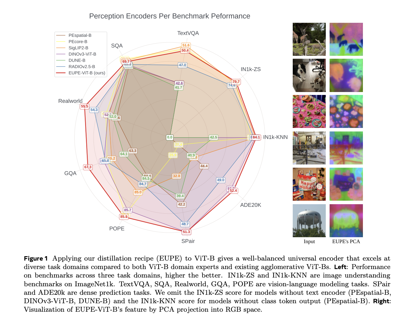Running powerful AI on your smartphone isn’t just a hardware problem — it’s a model architecture problem. Most state-of-the-art vision encoders are enormous, and when you trim them down to fit on an edge device, they lose the capabilities that made them useful in the first place. Worse, specialized models tend to excel at one type of task — image classification, say, or scene segmentation — but fall apart when you ask them to do something outside their lane. Meta’s AI research teams are now proposing a different path. They introduced the Efficient Universal Perception Encoder (EUPE): a compact vision encoder that handles diverse vision tasks simultaneously without needing to be large. The Core Problem: Specialists vs. Generalists To understand why EUPE matters, it helps to understand how vision encoders work and why specialization is a problem. A vision encoder is the part of a computer vision model that converts raw image pixels into a compact representation — a set of feature vectors — that downstream tasks (like classification, segmentation, or answering questions about an image) can use. Think of it as the ‘eyes’ of an AI pipeline. Modern foundation vision encoders are trained with specific objectives, which gives them an edge in particular domains. For example: CLIP and SigLIP 2 are trained on text-image pairs. They’re strong at image understanding and vision-language modeling, but their performance on dense prediction tasks (which require spatially precise, pixel-level features) often falls below expectations. DINOv2 and its successor DINOv3 are self-supervised models that learn exceptional structural and geometric descriptors, making them strong at dense prediction tasks like semantic segmentation and depth estimation. But they lack satisfactory vision-language capabilities. SAM (Segment Anything Model) achieves impressive zero-shot segmentation through training on massive segmentation datasets, but again falls short on vision-language tasks. For an edge device — a smartphone or AR headset — that needs to handle all of these task types simultaneously, the typical solution is to deploy multiple encoders at once. That quickly becomes compute-prohibitive. The alternative is accepting that a single encoder will underperform in several domains. Previous Attempts: Why Agglomerative Methods Fell Short on Efficient Backbones Researchers have tried to combine the strengths of multiple specialist encoders through a family of methods called agglomerative multi-teacher distillation. The basic idea: train a single student encoder to simultaneously mimic several teacher models, each of which is a domain expert. AM-RADIO and its follow-up RADIOv2.5 are perhaps the most well-known examples of this approach. They showed that agglomerative distillation can work well for large encoders — models with more than 300 million parameters. But the EUPE research demonstrates a clear limitation: when you apply the same recipe to efficient backbones, the results degrade substantially. RADIOv2.5-B, the ViT-B-scale variant, has significant gaps compared to domain experts on dense prediction and VLM tasks. Another agglomerative method, DUNE, merges 2D vision and 3D perception teachers through heterogeneous co-distillation, but similarly struggles at the efficient backbone scale. The root cause, the research team argue, is capacity. Efficient encoders simply don’t have enough representational capacity to directly absorb diverse feature representations from multiple specialist teachers and unify them into a universal representation. Trying to do so in one step produces a model that is mediocre across the board. EUPE’s Answer: Scale Up First, Then Scale Down The key insight behind EUPE is a principle named ‘first scaling up and then scaling down.‘ Instead of distilling directly from multiple domain-expert teachers into a small student, EUPE introduces an intermediate model: a large proxy teacher with enough capacity to unify the knowledge from all the domain experts. This proxy teacher then transfers its unified, universal knowledge to the efficient student through distillation. The full pipeline has three stages: Stage 1 — Multi-Teacher Distillation into the Proxy Model. Multiple large foundation encoders serve as teachers simultaneously, processing label-free images at their native resolutions. Each teacher outputs a class token and a set of patch tokens. The proxy model — a 1.9B parameter model trained with 4 register tokens — is trained to mimic all teachers at once. The selected teachers are: PEcore-G (1.9B parameters), selected as the domain expert for zero-shot image classification and retrieval PElang-G (1.7B parameters), which the research team found is crucial for vision-language modeling, particularly OCR performance DINOv3-H+ (840M parameters), selected as the domain expert for dense prediction To stabilize training, teacher outputs are normalized by subtracting the per-coordinate mean and dividing by the standard deviation, computed once over 500 iterations before training begins and kept fixed thereafter. This is deliberately simpler than the complex PHI-S normalization used in RADIOv2.5, and avoids the cross-GPU memory overhead of computing normalization statistics on-the-fly. Stage 2 — Fixed-Resolution Distillation into the Efficient Student. With the proxy model now serving as a single universal teacher, the target efficient encoder is trained at a fixed resolution of 256×256. This fixed resolution makes training computationally efficient, allowing a longer learning schedule: 390,000 iterations with a batch size of 8,192, cosine learning rate schedule, a base learning rate of 2e-5, and weight decay of 1e-4. Standard data augmentation applies: random resized cropping, horizontal flipping, color jittering, Gaussian blur, and random solarization. For the distillation loss, the class token loss uses cosine similarity, while the patch token loss combines cosine similarity (weight α=0.9) and smooth L1 loss (weight β=0.1). Adapter head modules — 2-layer MLPs — are appended to the student to match each teacher’s feature dimension. If student and teacher patch token spatial dimensions differ, 2D bicubic interpolation is applied to align them. Stage 3 — Multi-Resolution Finetuning. Starting from the Stage 2 checkpoint, the student undergoes a shorter finetuning phase using an image pyramid of three scales: 256, 384, and 512. The student and the proxy teacher independently and randomly select one scale per iteration — so they may process the same image at different resolutions. This forces the student to learn representations that generalize across spatial granularities, accommodating downstream tasks that operate at various resolutions. This stage runs for 100,000 iterations at a batch size of 4,096 and base learning rate of 1e-5. It is intentionally shorter because multi-resolution training is computationally costly — one iteration in Stage 3 takes roughly twice as long as in Stage 2. Training Data. All three stages use the same DINOv3 dataset, LVD-1689M, which provides balanced coverage of visual concepts from the web alongside high-quality public datasets including ImageNet-1k. The sampling probability from ImageNet-1k is 10%, with the remaining 90% from LVD-1689M. In an ablation study, training on LVD-1689M consistently outperformed training on MetaCLIP (2.5B images) on nearly all benchmarks — despite MetaCLIP being approximately 800M images larger — indicating higher data quality in LVD. An Important Negative Result: Not All Teachers Combine Well One of the more practically useful findings concerns teacher selection. Intuitively, adding more strong teachers should help. But the research team found that including SigLIP2-G alongside PEcore-G and DINOv3-H+ substantially degrades OCR performance. At the proxy model level, TextVQA drops from 56.2 to 53.2; at the ViT-B student level, it drops from 48.6 to 44.8. The research teams’ hypothesis: having two CLIP-style models (PEcore-G and SigLIP2-G) in the teacher set simultaneously causes feature incompatibility. PElang-G, a language-focused model derived from PEcore-G through alignment with language models, proved a far better complement — improving OCR and general VLM performance without sacrificing image understanding or dense prediction. What the Numbers Say The ablation studies validate the three-stage design. Distilling directly from multiple teachers to an efficient student (“Stage 2 only”) yields poor VLM performance, especially on OCR-type tasks, and poor dense prediction. Adding Stage 1 (the proxy model) significantly improves VLM tasks — TextVQA rises from 46.8 to 48.3, and Realworld from 53.5 to 55.1 — but still lags on dense tasks. Stage 1+3 (skipping Stage 2) gives the strongest dense prediction results (SPair: 53.3, NYUv2: 0.388) but leaves VLM gaps and is costly to run for a full schedule. The full three-stage pipeline achieves the best overall balance. On the main ViT-B benchmark, EUPE-ViT-B consistently stands out: Image understanding: EUPE achieves 84.1 on IN1k-KNN, outperforming PEcore-B (79.7), SigLIP2-B (83.2), and DINOv3-ViT-B (83.0). On IN1k-ZS (zero-shot), it scores 79.7, outperforming PEcore-B (78.4) and SigLIP2-B (78.2). Dense prediction: EUPE achieves 52.4 mIoU on ADE20k, outperforming the dense prediction expert DINOv3-ViT-B (51.8). On SPair-71k semantic correspondence, it scores 51.3, matching DINOv3-ViT-B. Vision-language modeling: EUPE outperforms both PEcore-B and SigLIP2-B on RealworldQA (55.5 vs. 52.9 and 52.5) and GQA (67.3 vs. 65.6 and 65.2), while staying competitive on TextVQA, SQA, and POPE. Vs. agglomerative methods: EUPE outperforms RADIOv2.5-B and DUNE-B on all VLM tasks and most dense prediction tasks by significant margins. What the Features Actually Look Like The research also includes qualitative feature visualization using PCA projection of patch tokens into RGB space — a technique that reveals the spatial and semantic structure an encoder has learned. The results are telling: PEcore-B and SigLIP2-B patch tokens contain semantic information but are not spatially consistent, leading to noisy representations. DINOv3-ViT-B has highly sharp, semantically coherent features, but lacks fine-grained discrimination (food and plates end up with similar representations in the last row example). RADIOv2.5-B features are overly sensitive, breaking semantic coherence — for example, black dog fur merges visually with the background. EUPE-ViT-B combines semantic coherence, fine granularity, complex spatial structure, and text awareness simultaneously — capturing the best qualities across all domain experts at once. A Full Family of Edge-Ready Models EUPE is a complete family spanning two architecture types: ViT family: ViT-T (6M parameters), ViT-S (21M), ViT-B (86M) ConvNeXt family: ConvNeXt-Tiny (29M), ConvNeXt-Small (50M), ConvNeXt-Base (89M) All models are under 100M parameters. Inference latency is measured on iPhone 15 Pro CPU via ExecuTorch-exported models. At 256×256 resolution: ViT-T runs in 6.8ms, ViT-S in 17.1ms, and ViT-B in 55.2ms. The ConvNeXt variants have lower FLOPs than ViTs of similar size, but do not necessarily achieve lower latency on CPU — because convolutional operations are often less efficient on CPU architecture compared to the highly optimized matrix multiplication (GEMM) operations used in ViTs. For the ConvNeXt family, EUPE consistently outperforms the DINOv3-ConvNeXt family of the same sizes across Tiny, Small, and Base variants on dense prediction, while also unlocking better VLM capability — particularly for OCR and vision-centric tasks — that DINOv3-ConvNeXt entirely lacks. Key Takeaways One encoder to rule them all. EUPE is a single compact vision encoder (under 100M parameters) that matches or outperforms specialized domain-expert models across image understanding, dense prediction, and vision-language modeling — tasks that previously required separate, dedicated encoders. Scale up before you scale down. The core innovation is a three-stage “proxy teacher” distillation pipeline: first aggregate knowledge from multiple large expert models into a 1.9B parameter proxy, then distill from that single unified teacher into an efficient student — rather than directly distilling from multiple teachers at once. Teacher selection is a design decision, not a given. Adding more teachers doesn’t always help. Including SigLIP2-G alongside PEcore-G degraded OCR performance significantly. PElang-G turned out to be the right VLM complement — a finding with direct practical implications for anyone building multi-teacher distillation pipelines. Built for real edge deployment. The full EUPE family spans six models across ViT and ConvNeXt architectures. The smallest, ViT-T, runs in 6.8ms on iPhone 15 Pro CPU. All models are exported via ExecuTorch and available on Hugging Face — ready for on-device integration, not just benchmarking. Data quality beats data quantity. In ablation experiments, training on LVD-1689M outperformed training on MetaCLIP across nearly all benchmarks — despite MetaCLIP containing roughly 800 million more images. A useful reminder that bigger datasets don’t automatically mean better models. Check out the Paper, Model Weight and Repo.  Also, feel free to follow us on Twitter and don’t forget to join our 120k+ ML SubReddit and Subscribe to our Newsletter. Wait! are you on telegram? now you can join us on telegram as well. Need to partner with us for promoting your GitHub Repo OR Hugging Face Page OR Product Release OR Webinar etc.? Connect with us The post Meta AI Releases EUPE: A Compact Vision Encoder Family Under 100M Parameters That Rivals Specialist Models Across Image Understanding, Dense Prediction, and VLM Tasks appeared fir […]

An Implementation Guide to Running NVIDIA Transformer Engine with Mixed Precision, FP8 Checks, Benchmarking, and Fallback ExecutionIn this tutorial, […]

The one piece of data that could actually shed light on your job and AIThis story originally appeared in The Algorithm, our weekly newsletter on […]

Announcing the OpenAI Safety FellowshipA pilot program to support independent safety and alignment research and develop the next generation of talent

Industrial policy for the Intelligence AgeExplore our ambitious, people-first industrial policy ideas for the AI era—focused on expanding opportunity, sharing prosperity, and building resilient institutions as advanced intelligence evolves.

Google’s Gemma 4: Is it the Best Open-Source Model of 2026?The latest set of open-source models from Google are here, the Gemma 4 family has […]

RightNow AI Releases AutoKernel: An Open-Source Framework that Applies an Autonomous Agent Loop to GPU Kernel Optimization for Arbitrary PyTorch Models Writing fast GPU code is one of the most grueling specializations in machine learning engineering. Researchers from RightNow AI want to automate it entirely. The RightNow AI research team has released AutoKernel, an open-source framework that applies an autonomous LLM agent loop to GPU kernel optimization for arbitrary PyTorch models. The approach is straightforward: give it any model before you go to bed, and wake up to faster Triton kernels — no GPU expertise required. Why GPU Kernels Are So Hard to Optimize A GPU kernel is a function that runs in parallel across thousands of GPU cores. When you run a transformer model like LLaMA or GPT-2, the bulk of compute time is spent inside kernels for operations like matrix multiplication (matmul), softmax, layer normalization, and attention. These kernels live in libraries like cuBLAS and cuDNN, or get generated automatically by PyTorch’s compilation pipeline. The problem is that squeezing maximum performance out of these kernels requires reasoning simultaneously about arithmetic intensity, memory coalescing, register pressure, tile sizes, warp-level synchronization, and tensor core instruction selection — a combination of skills that takes years to develop. A single high-performance matmul kernel may involve 200+ lines of CUDA or Triton code with dozens of interdependent parameters. This expertise is scarce, and the manual tuning process scales poorly as model architectures evolve. The benchmark suite KernelBench, which evaluates frontier LLMs on 250 GPU kernel problems, found that even the best models matched PyTorch baseline performance in fewer than 20% of cases using one-shot generation. AutoKernel was built directly in response to that gap. The Loop: Edit, Benchmark, Keep or Revert AutoKernel’s core insight is that an expert kernel engineer’s workflow is itself a simple loop: write a candidate, benchmark it, keep improvements, discard regressions, repeat. The framework mechanizes this loop. An LLM agent modifies a single file — kernel.py — a fixed benchmark harness verifies correctness and measures throughput, and the result determines whether the change persists. Crucially, every experiment maps to a git commit. Kept experiments advance the branch; reverted experiments are erased cleanly with git reset. The entire history is browsable with standard git tools, and experiment results are logged to a plain tab-separated results.tsv file — dependency-free, human-readable, and trivially parseable by the agent. Each iteration takes approximately 90 seconds — 30 seconds for correctness checking, 30 seconds for performance benchmarking via Triton’s do_bench, and 30 seconds for agent reasoning and code modification. At roughly 40 experiments per hour, an overnight 10-hour run yields 300 to 400 experiments across multiple kernels. This design draws directly from Andrej Karpathy’s autoresearch project, which demonstrated that an AI agent running a keep/revert loop on LLM training code could discover 20 optimizations across 700 experiments in two days on a single GPU. AutoKernel transplants this loop to kernel code, with a different search space and a correctness-gated benchmark as the evaluation function instead of validation loss. The agent reads a 909-line instruction document called program.md, which encodes expert knowledge into a six-tier optimization playbook. The tiers progress from block size tuning (sweeping tile dimensions through powers of 2, adjusting num_warps and num_stages) through memory access patterns (coalesced loads, software prefetching, L2 swizzling), compute optimizations (TF32 accumulation, epilogue fusion), advanced techniques (split-K, persistent kernels, Triton autotune, warp specialization), architecture-specific strategies (TMA on Hopper, cp.async on Ampere, adjusted sizes for L4/RTX), and finally kernel-specific algorithms like online softmax for attention and Welford’s algorithm for normalization. The instruction document is intentionally comprehensive so the agent can run 10+ hours without getting stuck. Profiling First, Optimizing Where It Matters Unlike prior work that treats kernel problems in isolation, AutoKernel starts from a complete PyTorch model. It uses torch.profiler with shape recording to capture per-kernel GPU time, then ranks optimization targets using Amdahl’s law — the mathematical principle that the overall speedup you can achieve is bounded by how much of the total runtime that component represents. A 1.5× speedup on a kernel consuming 60% of total runtime yields a 1.25× end-to-end gain. The same speedup on a kernel consuming 5% of runtime yields only 1.03×. The profiler detects GPU hardware from a database of known specifications covering both NVIDIA (H100, A100, L40S, L4, A10, RTX 4090/4080/3090/3080) and AMD (MI300X, MI325X, MI350X, MI355X) accelerators. For unknown GPUs, it estimates peak FP16 throughput from SM count, clock rate, and compute capability — making the system usable across a wider range of hardware than just the latest NVIDIA offerings. The orchestrator (orchestrate.py) transitions from one kernel to the next when any of four conditions are met: five consecutive reverts, 90% of GPU peak utilization reached, a two-hour elapsed time budget, or a 2× speedup already achieved on that kernel. This prevents the agent from spending excessive time on kernels with diminishing returns while higher-impact targets wait. Five-Stage Correctness Harness Performance without correctness is useless, and AutoKernel is particularly thorough on this front. Every candidate kernel passes through five validation stages before any speedup is recorded. Stage 1 runs a smoke test on a small input to catch compilation errors and shape mismatches in under a second. Stage 2 sweeps across 8 to 10 input configurations and three data types — FP16, BF16, and FP32 — to catch size-dependent bugs like boundary handling and tile remainder logic. Stage 3 tests numerical stability under adversarial inputs: for softmax, rows of large identical values; for matmul, extreme dynamic range; for normalization, near-zero variance. Stage 4 verifies determinism by running the same input three times and requiring bitwise identical outputs, which catches race conditions in parallel reductions and non-deterministic atomics. Stage 5 tests non-power-of-two dimensions like 1023, 4097, and 1537 to expose masking bugs and tile remainder errors. Tolerances are dtype-specific: FP16 uses atol = 10⁻², BF16 uses 2 × 10⁻², and FP32 uses 10⁻⁴. In the paper’s full evaluation across 34 configurations on an NVIDIA H100, all 34 passed correctness with zero failures across eager, compiled, and custom kernel outputs. Dual Backend: Triton and CUDA C++ AutoKernel supports both Triton and CUDA C++ backends within the same framework. Triton is a Python-like domain-specific language that compiles JIT in 1 to 5 seconds, making it ideal for rapid iteration — the agent can modify block sizes, warp counts, pipeline stages, accumulator precision, and loop structure. Triton routinely reaches 80 to 95% of cuBLAS throughput for matmul. CUDA C++ is included for cases requiring direct access to warp-level primitives, WMMA tensor core instructions (using 16×16×16 fragments), vectorized loads via float4 and half2, bank-conflict-free shared memory layouts, and double buffering. Both backends expose the same kernel_fn() interface, so the benchmark infrastructure runs identically regardless of backend. The system covers nine kernel types spanning the dominant operations in modern transformer architectures: matmul, flash_attention, fused_mlp, softmax, layernorm, rmsnorm, cross_entropy, rotary_embedding, and reduce. Each has a PyTorch reference implementation in reference.py serving as the correctness oracle, and the benchmark computes throughput in TFLOPS or GB/s alongside roofline utilization against detected GPU peak. Benchmark Results on H100 Measured on an NVIDIA H100 80GB HBM3 GPU (132 SMs, compute capability 9.0, CUDA 12.8) against PyTorch eager and torch.compile with max-autotune, the results for memory-bound kernels are significant. RMSNorm achieves 5.29× over eager and 2.83× over torch.compile at the largest tested size, reaching 2,788 GB/s — 83% of H100’s 3,352 GB/s peak bandwidth. Softmax reaches 2,800 GB/s with a 2.82× speedup over eager and 3.44× over torch.compile. Cross-entropy achieves 2.21× over eager and 2.94× over torch.compile, reaching 2,070 GB/s. The gains on these kernels come from fusing multi-operation ATen decompositions into single-pass Triton kernels that minimize HBM (High Bandwidth Memory) traffic. AutoKernel outperforms torch.compile on 12 of the 16 representative configurations benchmarked in the paper, despite torch.compile with max-autotune running its own Triton autotuning. TorchInductor’s generic fusion and autotuning does not always find the specialized tiling and reduction strategies that kernel-specific implementations exploit. Matmul is notably harder — PyTorch’s cuBLAS backend is extensively tuned per GPU architecture. The Triton starter reaches 278 TFLOPS, well below cuBLAS. However, at the 2048³ size, AutoKernel beats torch.compile by 1.55×, demonstrating that TorchInductor’s matmul autotuning is not always optimal either. Closing the cuBLAS gap remains the primary target for continued agent iteration. In community deployment, an AutoKernel-optimized kernel took first place on the vectorsum_v2 B200 leaderboard with a latency of 44.086µs, outperforming the second-place entry at 44.249µs and third place at 46.553µs. A community user also reported that a single AutoKernel prompt — requiring approximately three minutes of agent interaction — produced a Triton FP4 matrix multiplication kernel that outperforms CUTLASS by 1.63× to 2.15× across multiple shapes on H100. CUTLASS represents hand-optimized C++ template code specifically designed for NVIDIA tensor cores, making this result particularly notable. Key Takeaways AutoKernel turns weeks of expert GPU tuning into an overnight autonomous process. By mechanizing the write-benchmark-keep/revert loop that expert kernel engineers already follow, the system runs 300 to 400 experiments per overnight session on a single GPU without any human intervention. Correctness is non-negotiable before any speedup is recorded. Every candidate kernel must pass a five-stage harness covering smoke tests, shape sweeps across 10+ configurations, numerical stability under adversarial inputs, determinism verification, and non-power-of-two edge cases — eliminating the risk of the agent “optimizing” its way to incorrect outputs. Memory-bound kernels see the biggest gains over both PyTorch eager and torch.compile. On an NVIDIA H100, AutoKernel’s Triton kernels achieve 5.29× over eager on RMSNorm, 2.82× on softmax, and 2.21× on cross-entropy — with the gains coming from fusing multi-operation ATen decompositions into single-pass kernels that minimize HBM traffic. Amdahl’s law drives where the agent spends its time. Rather than optimizing kernels in isolation, AutoKernel profiles the entire PyTorch model and allocates effort proportionally to each kernel’s share of total GPU runtime — ensuring that improvements compound at the model level, not just the kernel level. Check out the Paper and Repo.  Also, feel free to follow us on Twitter and don’t forget to join our 120k+ ML SubReddit and Subscribe to our Newsletter. Wait! are you on telegram? now you can join us on telegram as well. Need to partner with us for promoting your GitHub Repo OR Hugging Face Page OR Product Release OR Webinar etc.? Connect with us The post RightNow AI Releases AutoKernel: An Open-Source Framework that Applies an Autonomous Agent Loop to GPU Kernel Optimization for Arbitrary PyTorch Models appeared first on Mark […]